M.Tech U -V Fabrication

NANOCHEMISTRY

NANO FABRICATION-1

NANO FABRICATION-2,

Crystal Growth and Wafer Preparation


Unit-V   Fabrication:Crystal growth and wafer preparation, Defects, Clean room concept, Wafer cleaning techniques, Oxidation, Diffusion, Epitaxy, Ion implantation, Metallization, Lithography, Etching, Masking sequences and bipolar and MOS device fabrication process flow, Integration of unit process, Process modeling, Topological design rules, Passive device such as registers and capacitors and their non idealities, Fabrication of nanoelectronics structures.


M.Tech U-IV Applied chemistry of nanomaterials

Unit-IV   Applied chemistry of nanomaterials:Application to fundamenatal studies. Industrial applications: Photographic materials, Ceramic materials, Magnetic particles for recording media, Catalysts, Fuel cells electrocatalysis,Pigments, Nanostructured materials as new chemical reagents, Nanocomposite polymers, Fluids, inks and dyes, Block copolymers and dendrimers. Analytical and Environmental chemistry of nanoparticles.


Nanomaterials and their Applications

Nanomaterial Applications using Carbon Nanotubes

Applications being developed for carbon nanotubes include adding antibodies to nanotubes to form bacteria sensors, making a composite with nanotubes that bend when electric voltage is applied bend the wings of morphing aircraft, adding boron or gold to nanotubes to trap oil spills, include smaller transistors, coating nanotubes with silicon  to make anodes the can increase the capacity of Li-ion batteries by up to 10 times.

Nanomaterial Applications using Graphene

Applications being developed for graphene include using graphene sheets as electodes in ultracapacitors which will have as much storage capacity as batteries but will be able to recharge in minutes, attaching strands of DNA to graphene to form sensors for rapid disease diagnostics, replacing indium in flat screen TVs and making high strenght composite materials.

Nanomaterial Applications using Nanocomposites

Applications being developed for nanocomposites include a nanotube-polymer nanocomposite to form a scaffold which speeds up replacement of broken bones, making a graphene-epoxy nanocomposite with very high strenght-to-weight ratios, a nanocomposite made from cellulous and nanotubes used to make a flexible battery.

Nanomaterial Applications using Nanofibers

Applications being developed for nanofibers include stimulating the production of cartilage in damaged joints, piezoelectric nanofibers that can be woven into clothing to produce electricty for cell phones or other devices, carbon nanofibers that can improve the preformance flame retandant in funiture.

Nanomaterial Applications using Nanoparticles

Applications being developed for nanoparticles include deliver chemotherapy drugs directly to cancer tumors, resetting the immune system to prevent autoimmune diseases, delivering drugs to damaged regions of arteries to fight cardiovascular disease, create photocatalysts that produce hydrogen from water, reduce the cost of producing fuel cells and solar cells, clean up oil spills, water pollution and air pollution.

Nanomaterial Applications using Nanowires

Applications being developed for carbon nanotubes include using zinc oxide nanowires in a flexible solar cell, silver chloride nanowires to decompose organic molecules in polluted water, using nanowires made from iron and nickel to make dense computer memory – called “race track memo


Nanomaterials and their Applications

Nanomaterial Applications using Carbon Nanotubes

Applications being developed for carbon nanotubes include adding antibodies to nanotubes to form bacteria sensors, making a composite with nanotubes that bend when electric voltage is applied bend the wings of morphing aircraft, adding boron or gold to nanotubes to trap oil spills, include smaller transistors, coating nanotubes with silicon  to make anodes the can increase the capacity of Li-ion batteries by up to 10 times.


The properties of carbon nanotubes have caused researchers and companies to consider using them in several fields.  The following survey of carbon nanotube applications introduces many of these uses.

Carbon Nanotubes and Energy

Researchers at the University of Delaware have demonstarted increased energy density for capacitors whit the use of carbon nanotubes in 3-D structured electrodes.

Researchers at North Carolina State University have demonstrated the use of silicon coated carbon nanotubes in anodes for Li-ion batteries. They are predicting that the use of silicon can increase the capacity of Li-ion batteries by up to 10 times. However silicon expands during a batteries discharge cycle, which can damage silicon based anodes. By depositing silicon on nanotubes aligned parallel to each other the researchers hope to prevent damage to the anode when the silicon expands.

Researchers at Los Alamos National Laboratory have demonstrated a catalyst made from nitrogen-doped carbon-nanotubes, instead of platinum. The researchers believe this type of catalyst could be used in Lithium-air batteries, which can store up to 10 times as much energy as lithium-ion batteries.

Researchers at Rice University have developed electrodes made from carbon nanotubes grown on graphene with very high surface area and very low electrical resistance. The researchers first grow graphene on a metal substrate then grow carbon nanotubes on the graphene sheet. Because the base of each nanotube is bonded, atom to atom, to the graphene sheet the nanotube-graphene structure is essentially one molecule with a huge surface area.

Using carbon nanotubes in the cathode layer of a battery that can be produced on almost any surface. The battery can be formed by simply spraying layers of paint containing the components needed for each part of the battery.

Carbon nanotubes can perform as a catalyst in a fuel cell, avoiding the use of expensive platinum on which most catalysts are based. Researchers have found that incorporating nitrogen and iron atoms into the carbon lattice of nanotubes results in nanotubes with catalytic properties.

Carbon Nanotubes In Healthcare

Researchers are improving dental implants by adding nanotubes to the surface of the implant material. They have shown that bone adheres better to titanium dioxide nanotubes than to the surface of standard titanium implants. As well they have demonstrated to the ability to load the nanotubes with anti-inflammatory drugs that can be applied directly to the area around the implant.

Reseachers at MIT have developed a sensor using carbon nanotubes embedded in a gel; that can be injected under the skin to monitor the level of nitric oxide in the bloodstream. The level of nitric oxide is important because it indicates inflamation, allowing easy monitoring of imflammatory diseases. In tests with laboratory mice the sensor remained functional for over a year.

Researchers have demonstrated artificial muscles composed of yarn woven with carbon nanotubes and filled with wax. Tests have shown that the artificial muscles can lift weights that are 200 times heavier than natural muscles of the same size.

Nanotubes bound to an antibody that is produced by chickens have been shown to be useful in lab tests to destroy breast cancer tumors. The antibody-carrying nanotubes are attracted to proteins produced by one type of breast cancer cell. Once attached to these cells, the nanotubes absorb light from an infrared laser, incinerating the nanotubes and the attached tumor.

Researchers at the University of Connecticut have developed a sensor that uses nanotubes and gold nanoparticles to detect proteins that indicate the presence of oral cancer. Tests have shown this sensor to be accurate and it provides results in less than an hour.

Carbon Nanotubes and the Environment

Carbon nanotubes are being developed to clean up oil spills. Researchers have found that adding boron atoms during the growth of carbon nanotubes causes the nanotubes to grow into a sponge like material that can absorb many times it’s weight in oil. These nanotube sponges are made to be magnetic, which should make retrieval of them easier once they are filled with oil.

Carbon nanotubes can be used as the pores in membranes to run reverse osmosis desalination plants. Water molecules pass through the smoother walls of carbon nanotubes more easily than through other types of nanopores, which requires less power. Other researchers are using carbon nanotubes to develope small, inexpensive water purification devices needed in developing countries.

Sensors using carbon nanotube detection elements are capable of detecting a range of chemical vapors. These sensors work by reacting to the changes in the resistance of a carbon nanotube in the presence of a chemical vapor.

Researchers at the Technische Universität München have demonstrated a method of spraying carbon nanotubes onto flexible plastic surfaces to produce sensors. The researchers believe that this method could produce low cost sensors on surfaces such as the plastic film wrapping food, so that the sensor could detect spoiled food.

An inexpensive nanotube-based sensor can detect bacteria in drinking water. Antibodies sensitive to a particular bacteria are bound to the nanotubes, which are then deposited onto a paper strip. When the bacteria is present it attaches to the antibodies, changing the spacing between the nanotubes and the resistance of the paper strip containing the nanotubes.

Carbon nanotubes tipped with gold nanoparticles can be used to trap oil drops polluting water. Since the gold end is attracted to water while the carbon end is attracted to oil. Therefore the nanotubes form spheres surrounding oil droplets with the carbon end pointed in, toward the oil, and the gold end pointing out, toward the water.

Carbon Nanotubes Effecting Materials

Researchers  are developing materials, such as a carbon nanotube-based composite developed by NASA that bends when a voltage is applied. Applications include the application of an electrical voltage to change the shape (morph) of aircraft wings and other structures. This video from NASA gives you an idea of what a futuristic morphing aircraft might look like.

Researchers have found that carbon nanotubes can fill the voids that occur in conventional concrete. These voids allow water to penetrate concrete causing cracks, but including nanotubes in the mixstops the cracks from forming.

Researchers at MIT have developed a method  to add carbon nanotubes aligned perpendicular to the carbon fibers, called nanostiching. They believe that having the nanotubes perpendicular to the carbon fibers help hold the fibers together, rather than depending upon epoxy, and significanly improve the properties of the composite.

Avalon Aviation incorporated carbon  nanotubes in a carbon fiber composite engine cowling on an aerobatic aircraft to increase the strength to weight ratio. The engine cowling is highly stressed components in this aircraft, adding carbon nanotubes to the composite allowed them to reduce the weight without weakening the component.

Carbon Nanotubes and Electronics

Building transistors from carbon nanotubes enables minimum transistor dimensions of a few nanometers and the development of techniques to manufacture integrated circuits built with nanotube transistors.

Researchers at Stanford University have demonstrated a method to make functioning integrated circuits using carbon nanotubes. In order to make the circuit work they developed methods to remove metallic nanotubes, leaving only semiconducting nanotubes, as well as an algorithm to deal with misaligned nanotubes. The demonstration circuit they fabricated in the university labs contains 178 functioning transistors.

Other applications in this area include:

Carbon Nanotube Company Directory

Company Products
Nano Lab Functionalizied nanotubes and nanotube arrays
Bayer Material Science Carbon nanotubes
Cheap Tubes Carbon nanotubes


Nanomaterial Applications using Graphene

Applications being developed for graphene include using graphene sheets as electodes in ultracapacitors which will have as much storage capacity as batteries but will be able to recharge in minutes, attaching strands of DNA to graphene to form sensors for rapid disease

diagnostics, replacing indium in flat screen TVs and making high strenght composite materials.

The properties of graphene, carbon sheets that are only one atom thick, have caused researchers and companies to consider using this material in several fields. The following survey of research activity introduces you to many potential applications of graphene.

A Survey of Applications:

Hydrogen production without platimum. Researchers have demonstrated a catalyst made fromgraphene doped with cobalt can be used to produce hydrogen from water. The researchers at looking at this method as a low cost replacement for platimum based catalysts.

Lower cost of display screens in mobile devices. Researchers have found that graphene can replace indium-based electrodes in organic light emitting diodes (OLED). These diodes are used in electronic device display screens which require low power consumption. The use of graphene instead of indium not only reduces the cost but eliminates the use of metals in the OLED, which may make devices easier to recycle.

Lithium-ion batteries that recharge faster. These batteries use graphene on the surface of the anode surface. Defects in the graphene sheet (introduced using a heat treatment) provide pathways for the lithium ions to attach to the anode substate. Studies have shown that the time needed to recharge a battery using the graphene anode is much shorter than with conventional lithium-ion batteries.

Ultracapacitors with better performance than batteries. These ultracapacitiors store electrons on graphene sheets, taking advantage of the large surface of graphene to provide increase the electrical power that can be stored in the capacitor. Researchers are projecting that these ultracapacitors will have as much electrical storage capacity as lithium ion batteries but will be able to be recharged in minutes instead of hours.

Components with higher strength to weight ratios. Researchers have found that adding graphene to epoxy composites may result in stronger/stiffer components than epoxy composites using a similar weight of carbon nanotubes. Graphene appears to bond better to the polymers in the epoxy, allowing a more effective coupling of the graphene into the structure of the composite. This property could result in the manufacture of components with high strength to weight ratio for such uses as windmill blades or aircraft components.

Storing hydrogen for fuel cell powered cars. Researchers have prepared graphene layers to increase the binding energy of hydrogen to the graphene surface in a fuel tank, resulting in a higher amount of hydrogen storage and therefore a lighter weight fuel tank. This could help in the development of practical hydrogen fueled cars.

Lower cost fuel cells. Researchers at Ulsan National Institute of Science and Technology have demonstrated how to produce edge-halogenated graphene nanoplatelets that have good catalytic properties. The researchers prepared the nanoplatelets by ball-milling graphene flakes in the presence of chlorine, bromine or iodine. They believe these halogenated nanoplatelets could be used as a replacement for expensive platinum catalystic material in fuel cells.

Low cost water desalination: Researchers have determined that graphene with holes the size of a nanometer or less can be used to remove ions from water. They believe this can be used to desalinate sea water at a lower cost than the reverse osmosis techniques currently in use.

Lightweight natural gas tanks: Researchers at Rice University have developed a composite material using plastic and graphene nanoribbons that block the passage of gas molecules. This material may be used in applications ranging from soft drink bottles to lightweight natural gas tanks.

More efficient dye sensitized solar cells. Researchers at Michigan Technological University have developed a honeycomb like structure of graphene in which the graphene sheets are held apart by lithium carbonate. They have used this “3D graphene” to replace the platinum in a dye sensitized solar cell and achieved 7.8 percent conversion of sunlight to electricity.

Electrodes with very high surface area and very low electrical resistance. Researchers at Rice University have developed electrodes made from carbon nanotubes grown on graphene. The researchers first grow graphene on a metal substrate then grow carbon nanotubes on the graphene sheet. Because the base of each nanotube is bonded, atom to atom, to the graphene sheet the nanotube-graphene structure is essentially one molecule with a huge surface area.

Lower cost solar cells: Researchers have built a solar cell that uses graphene as a electrode while using buckyballs and carbon nanotubes to absorb light and generate electrons; making a solar cell composed only of carbon. The intention is to eliminate the need for higher cost materials, and complicated manufacturing techniques needed for conventional solar cells.

Transistors that operate at higher frequency. The ability to build high frequency transistors with graphene is possible because of the higher speed at which electrons in graphene move compared to electrons in silicon. Researchers are also developing lithography techniques that can be used to fabricate integrated circuits based on graphene.

Sensors to diagnose diseases. These sensors are based upon graphene’s large surface area and the fact that molecules that are sensitive to particular diseases can attach to the carbon atoms in graphene. For example, researchers have found that graphene, strands of DNA, and fluorescent molecules can be combined to diagnose diseases. A sensor is formed by attaching fluorescent molecules to single strand DNA and then attaching the DNA to graphene.  When an identical single strand DNA combines with the strand on the graphene a double strand DNA if formed that floats off from the graphene, increasing the fluorescence level. This method results in a sensor that can detect the same DNA for a particular disease in a sample.

Membranes for more efficient separation of gases. These membranes are made from sheets ofgraphene in which nanoscale pores have been created. Because graphene is only one atom thick researchers believe that gas separation will require less energy than thicker membranes.

Chemical sensors effective at detecting explosives. These sensors contain sheets of graphene in the form of a foam which changes resistance when low levels of vapors from chemicals, such as ammonia, is present.

Graphene Company Directory

Graphene Company Product
Angstron Materials Graphene Supplier
Bluestone Global Tech Graphene Supplier
CrayoNano Semiconductor nanowires grown on graphene


Nanomaterial Applications using Nanocomposites

Applications being developed for nanocomposites include a nanotube-polymer nanocomposite to form a scaffold which speeds up replacement of broken bones, making a graphene-epoxy nanocomposite with very high strenght-to-weight ratios, a nanocomposite made from cellulous and nanotubes used to make a flexible battery.


nanocomposite is a matrix to which nanoparticles have been added to improve a particular property of the material. The properties of nanocomposites have caused researchers and companies to consider using this material in several fields.

A survey of  the applications of nanocomposites:

The following survey of nanocomposite applications introduces you to many of the uses being explored, including:

Producing batteries with greater power output. Researchers have developed a method to make anodes for lithium ion batteries from a composite formed with silicon nanospheres and carbon nanoparticles. The anodes made of the silicon-carbon nanocomposite make closer contact with the lithium electrolyte, which allows faster charging or discharging of power.

Speeding up the healing process for broken bones. Researchers have shown that growth of replacement bone is speeded up when a nanotube-polymer nanocomposite is placed as a kind of scaffold which guides growth of replacement bone. The researchers are conducting studies to better understand how this nanocomposite increases bone growth.

Producing structural components with a high strength-to-weight ratio.  For example an epoxy containing carbon nanotubes can be used to produce nanotube-polymer composite windmill blades. This results in a strong but lightweight blade, which makes longer windmill blades practical. These longer blades increase the amount of electricity generated by each windmill.

Using graphene to make composites with even higher strength-to-weight ratios. Researchers have found that adding graphene to epoxy composites may result in stronger/stiffer components than epoxy composites using a similar weight of carbon

nanotubes. Graphene appears to bond better to the polymers in the epoxy, allowing a more effective coupling of the graphene into the structure of the composite. This property could result in the manufacture of components with higher strength-to-weight ratios for such uses as windmill blades or aircraft components.

Making lightweight sensors with nanocomposites. A polymer-nanotube nanocomposite conducts electricity; how well it conducts depends upon the spacing of the nanotubes. This property allows patches of polymer-nanotube nanocomposite to act as stress sensors on windmill blades. When strong wind gusts bend the blades the nanocomposite will also bend. Bending changes the nanocomposite sensor’s electrical conductance, causing an alarm to be sounded. This alarm would allow the windmill to be shut down before excessive damage occurs.

Using nanocomposites to make flexible batteries. A nanocomposite of cellulous materials and nanotubes could be used to make a conductive paper. When this conductive paper is soaked in an electrolyte, a flexible battery is formed.

Making tumors easier to see and remove. Researchers are attempting to join magnetic nanoparticles and fluorescent nanoparticles in a nanocomposite particle that is both magnetic and fluorescent. The magnetic property of the nanocomposite particle makes the tumor more visible during an MRI procedure  done prior to surgery. The fluorescent property of the nanocomposite particle could help the surgeon to better see the tumor while operating.

Nanocomposite Company Directory

Company Product
Nanosonic Metal Rubber™ nanocomposites
InMat Nanocomposite coatings
Nanocyl EPOCYL™ epoxy resins reinforced with carbon nanotubes
MesaCoat Nanocomposite coatings
NanoComposites Nanocomposite materials

More Nanocomposite Companies


Nanomaterial Applications using Nanofibers

Applications being developed for nanofibers include stimulating the production of cartilage in damaged joints, piezoelectric nanofibers that can be woven into clothing to produce electricty for cell phones or other devices, carbon nanofibers that can improve the preformance flame retandant in funiture.


A nanofiber is a fiber with a diameter of 100 nanometers or less. The properties of nanofibers have caused researchers and companies to consider using this material in several fields.

A survey of the applications of nanofibers:

Researchers are using nanofibers to capture individual cancer cells circulating in the blood stream. They use nanofibers coated with antibodies that bind to cancer cells, trapping the cancer cell for analysis.

Nanofibers can stimulate the production of cartilage in damaged joints. Three different approaches to the use of nanofibers to stimulate cartilage are being taken by researchers at John Hopkins University, at Northwestern University and at the University of Pennsylvania.

Reseachers are using nanofibers to delivery thrapeutic drugs. The have developed an elastic material that is embedded with needle like carbon nanofibers. The material is intended to be used as balloons which are inserted next diseased tissue, and then inflated. When the balloon is inflated the carbon nanofibers penetrate diseased cells and delivery therapeutic drugs.

Researchers at MIT have used carbon nanofibers to make lithium ion battery electrodes that show four times the storage capacity of current lithium ion batteries.

The next step beyond lithium-ion batteries may be lithium sulfur batteries (the cathode contains the sulfur), which have the capability of storing several times the energy of lithium-ion  batteries. Researchers at Stanford University are using cathodes made up of carbon nanofibers encapsulating the sulfur.

Researchers are using nanofibers to make sensors that change color as they absorb chemical vapors. They plan to use these sensors to show when the absorbing material in a gas mask becomes saturated.

Researchers have developed piezoelectric nanofibers that are flexible enough to be woven into clothing. The fibers can turn normal motion into electricity to power your cell phone and other mobile electronic devices.

Flame retardant formed by coating the foam used in furniture with carbon nanofibers.


Nanomaterial Applications using Nanoparticles

Applications being developed for nanoparticles include deliver chemotherapy drugs directly to cancer tumors, resetting the immune system to prevent autoimmune diseases, delivering drugs to damaged regions of arteries to fight cardiovascular disease, create photocatalysts that produce hydrogen from water, reduce the cost of producing fuel cells and solar cells, clean up oil spills, water pollution and air pollution


Nanoparticles have one dimension that measures 100 nanometers or less. The properties of many conventional materials change when formed from nanoparticles. This is typically because nanoparticles have a greater surface area per weight than larger particles which causes them to be more reactive to some other molecules.

Nanoparticles are used, or being evaluated for use, in many fields. The list below introduces several of the uses under development.

Nanoparticle Applications in Medicine

The use of polymeric micelle nanoparticles to deliver drugs to tumors.

The use of polymer coated iron oxide nanoparticles to break up clusters of bacteria, possibly allowing more effective treatment of chronic bacterial infections.

The surface change of protein filled nanoparticles has been shown to affect the ability of the nanoparticle to stimulate immune responses. Researchers are thinking that these nanoparticles may be used in inhalable vaccines.

Researchers at Rice University have demonstrated that cerium oxide nanoparticles act as an antioxidant to remove oxygen free radicals that are present in a patient’s bloodstream following a traumatic injury. The nanoparticles absorb the oxygen free radicals and then release the oxygen in a less dangerous state, freeing up the nanoparticle to absorb more free radicals.

Researhers are developing ways to use carbon nanoparticles called nanodiamonds in medical applications. For example nanodiamonds with protein molecules attached can be used to increase bone growth around dental or joint implants.

Researchers are testing the use of chemotherapy drugs attached to nanodiamonds to treat brain tumors. Other researchers are testing the use of chemotherapy drugs attached to nanodiamonds to treat leukemia.

More about Nanotechnology in Medicine

Nanoparticle Applications in Manufacturing and Materials

Ceramic silicon carbide nanoparticles dispersed in magnesium produce a strong, lightweight material.

A synthetic skin, that may be used in prosthetics, has been demonstrated with both self healing capability and the ability to sense pressure. The material is a composite of nickel nanoparticles and a polymer. If the material is held together after a cut it seals together in about 30 minutes giving it a self healing ability. Also the electrical resistance of the material changes with pressure, giving it a sense ability like touch.

Silicate nanoparticles can be used to provide a barrier to gasses (for example oxygen), or moisture in a plastic film used for packaging. This could slow down the process of spoiling or drying out in food.

Zinc oxide nanoparticles can be dispersed in industrial coatings to protect wood, plastic, and textiles from exposure to UV rays.

Silicon dioxide crystalline nanoparticles can be used to fill gaps between carbon fibers, thereby strengthening tennis racquets.

Silver nanoparticles in fabric are used to kill bacteria, making clothing odor-resistant.

Nanoparticle Applications and the Environment

Researchers are using photocatalytic copper tungsten oxide nanoparticles to break down oil into biodegradable compounds. The nanoparticles are in a grid that provides high surface area for the reaction, is activated by sunlight and can work in water, making them useful for cleaning up oil spills.

Researchers are using gold nanoparticles embedded in a porous manganese oxide as a room temperature catalyst to breakdown volatile organic pollutants in air.

Iron nanoparticles are being used to clean up carbon tetrachloride pollution in ground water.

Iron oxide nanoparticles are being used to clean arsenic from water wells.

Nanoparticle Applications in Energy and Electronics

Researchers have used nanoparticles called nanotetrapods studded with nanoparticles of carbon to develop low cost electrodes for fuel cells. This electrode may be able to replace the expensive platinum needed for fuel cell catalysts.


Researchers at Georgia Tech, the University of Tokyo and Microsoft Research have developed a method to print prototype circuit boards using standard inkjet printers. Silver nanoparticle ink was used to form the conductive lines needed in circuit boards.

Combining gold nanoparticles with organic molecules creates a transistor known as a NOMFET (Nanoparticle Organic Memory Field-Effect Transistor). This transistor is unusual in that it can function  in a way similar to synapses in the nervous system.

catalyst using platinum-cobalt nanoparticles is being developed for fuel cells that produces twelve times more catalytic activity than pure platinum. In order to achieve this performance, researchers anneal nanoparticles to form them into a crystalline lattice, reducing the spacing between platinum atoms on the surface and increasing their reactivity.

Researchers have demonstrated that sunlight, concentrated on nanoparticles, can produce steam with high energy efficiency. The “solar steam device” is intended to be used in areas of developing countries without electricity for applications such as purifying water or disinfecting dental instruments.

A lead free solder reliable enough for space missions and other high stress environments using copper nanoparticles.

Silicon nanoparticles coating anodes of lithium-ion batteries can increase battery power and reduce recharge time.

Semiconductor nanoparticles are being applied in a low temperature printing process that enables the  manufacture of low cost solar cells.

A layer of closely spaced palladium nanoparticles is being used in a hydrogen sensor. Whenhydrogen is absorbed, the palladium nanoparticles swell, causing shorts between nanoparticles. These shorts lower the resistance of the palladium layer.

Nanoparticle Company Directory

Company Products
CytImmune Gold nanoparticles for targeted delivery of drugs to tumors
Invitrogen Qdots for medical imaging
Antaria Zinc oxide nanoparticles used in coatings to reduce UV exposure
Nanoledge Epoxy resins strengthened with nanoparticles


Nanomaterial Applications using Nanowires

Applications being developed for carbon nanotubes include using zinc oxide nanowires in a flexible solar cell, silver chloride nanowires to decompose organic molecules in polluted water, using nanowires made from iron and nickel to make dense computer memory – called “race track memory


The properties of nanowires have caused researchers and companies to consider using this material in several fields.

Nanowires Applications in Energy

Researchers at MIT have developed a solar cell using graphene coated with zinc oxide nanowires. The researchers believe that this method will allow the production of low cost flexible solar cells at high enough efficiency to be competive.

Sensors powered by electricity generated by piezoelectric zinc oxide nanowires. This could allowsmall, self contained, sensors powered by mechanical energy such as tides or wind

Researchers are using a method called Aerotaxy to grow semiconducting nanowires on gold nanoparticles. They plan to use self assembly techniques to align the nanowires on a substrate; forming a solar cell or other electrical devices. The gold nanoparticles replace the silicon substrate on which conventional semiconductor based solar cells are built.

Researchers at the Nies Bohr Institute have determined that sunlight can be concentrated in nanowires due to a resonance effect. This effect can result in more efficient solar cells, allowing more of the energy from the sun to be converted to electricity.

Using light absorbing nanowires embedded in a flexible polymer film is another method being developed to produce low cost flexible solar panels.

Researchers at Lawrence Berkeley have demonstrated an inexpensive process for making solar cells. These solar cells are composed of cadmium sulfide nanowires coated with copper sulfide.

Researchers at Stanford University have grown silicon nanowires on a stainless steel substrate and demonstrated that batteries using these anodes could have up to 10 times the power density of conventional lithium ion batteries. Using silicon nanowires, instead of bulk silicon fixes a problem of the silicon cracking, that has been seen on electrodes using bulk silicon. The cracking is caused because the silicon swells it absorbs lithium ions while being recharged, and contracts as the battery is discharged and the lithium ions leave the silicon. However the researchers found that while the silicon nanowires swell as lithium ions are absorbed during discharge of the battery and contract as the lithium ions leave during recharge of the battery the nanowires do not crack, unlike anodes that used bulk silicon.

Nanowire Applications in the Enviroment

Using silver chloride nanowires as a photocatalysis to decompose organic molecules in polluted water.

Using an electrified filter composed of silver nanowires, carbon nanotubes and cotton to kill bacteria in water.

Using nanowire mats to absorb oil spill

Nanowire Applications in Electronics

Using electrodes made from nanowires that would enable flat panel displays to be flexible as well as thinner than current flat panel displays.

Using nanowires to build transistors without p-n junctions.

Using nanowires made of an alloy of iron and nickel to create dense memory devices. By applying a current magnetized sections along the length of the wire. As the magnetized sections move along the wire, the data is read by a stationary sensor. This method is called race track memory.

Using silver nanowires embedded in a polymer to make conductive layers that can flex, without damaging the conductor.

Sensors using zinc oxide nano-wire detection elements capable of detecting

M.Tech U III The effect of chemistry of nanostructures

Unit-III  The effect of chemistry of nanostructures: Modification of nanoparticles, Langmuir Blodgett films, Self assembled surface films, Binding of molecules on solid substrate surfaces, Molecular nanostructures, Strategies of molecular construction, Synthetic supramolecules.


Modification of nanoparticles

Nanoparticles and nanocomposites are used in a wide range of applications in various fields, such as medicine, textiles, cosmetics, agriculture, optics, food packaging, optoelectronic devices, semiconductor devices, aerospace, construction and catalysis. Nanoparticles can be incorporated into polymeric nanocomposites. Polymeric nanocomposites consisting of inorganic nanoparticles and organic polymers represent a new class of materials that exhibit improved performance compared to their microparticle counterparts. It is therefore expected that they will advance the field of engineering applications. Incorporation of inorganic nanoparticles into a polymer matrix can significantly affect the properties of the matrix. The resulting composite might exhibit improved thermal, mechanical, rheological, electrical, catalytic, fire retardancy and optical properties. The properties of polymer composites depend on the type of nanoparticles that are incorporated, their size and shape, their concentration and their interactions with the polymer matrix. The main problem with polymer nanocomposites is the prevention of particle aggregation. It is difficult to produce monodispersed nanoparticles in a polymer matrix because nanoparticles agglomerate due to their specific surface area and volume effects. This problem can be overcome by modification of the surface of the inorganic particles. The modification improves the interfacial interactions between the inorganic particles and the polymer matrix. There are two ways to modify the surface of inorganic particles. The first is accomplished through surface absorption or reaction with small molecules, such as silane coupling agents, and the second method is based on grafting polymeric molecules through covalent bonding to the hydroxyl groups existing on the particles. The advantage of the second procedure over the first lies in the fact that the polymer-grafted particles can be designed with the desired properties through a proper selection of the species of the grafting monomers and the choice of grafting conditions.


Langmuir, Langmuir-Blodgett, Langmuir-Schaefer Technique

The Langmuir (L), Langmuir-Blodgett (LB) and Langmuir-Schaefer (LS) techniques enable fabrication and characterization of single molecule thick films with control over the packing density of molecules. They also enable the creation of multilayer structures with varying layer composition.

Langmuir, Langmuir-Blodgett, Langmuir-Schaefer—what is the difference?

When a monolayer is fabricated at the gas-liquid or liquid-liquid interface, the film is named Langmuir film. A Langmuir film can be deposited on a solid surface and is thereafter called Langmuir-Blodgett film (in the case of vertical deposition) or Langmuir-Schaefer film (in the case of horizontal deposition). Langmuir-Schaefer is often seen just as a variant of Langmuir-Blodgett deposition.

Langmuir film, Langmuir-Blodgett deposition, Langmuir-Schaefer deposition and multilayers obtained after repeated deposition.

Langmuir Troughs (or Langmuir film balance) are used for Langmuir film fabrication and characterization. Langmuir-Blodgett troughs are used for Langmuir-Blodgett or Langmuir-Schaefer deposition. All KSV NIMA Troughs are modular and when equipped with the right modules can be used for Langmuir film fabrication or characterization as well as Langmuir-Blodgett and Langmuir-Schaefer deposition.

The components of L and LB Troughs

Langmuir troughs include a set of barriers (2), a Langmuir trough top (3*) and a surface pressure sensor (4) as standard. The software-controlled barriers are placed at the interface and compress the monolayer. The trough top holds the liquid phase where monolayers are fabricated. The trough top is often made of hydrophobic material that improves sub-phase containment. The surface pressure sensor provides information about monolayer packing density.

Langmuir-Blodgett troughs include a set of barriers (2), a Langmuir-Blodgett trough top (3*), a surface pressure sensor (4) and a dipping mechanism (5) as standard. The Langmuir-Blodgett trough top holds the liquid phase and has a well in the center to allow space for solid substrate dipping through the monolayer. The dipping mechanism holds the solid substrate and enables controlled deposition cycle(s).

Please note that for Langmuir-Schaefer deposition, the Langmuir-Blodgett trough top is not always necessary and can in some cases be replaced by a Langmuir trough top.

KSV NIMA L & LB Trough modules

  1. Frame
  2. Barriers
  3. Trough top
  4. Surface pressure sensor
  5. Dipping mechanism (LB option)
  6. Interface unit

KSV NIMA troughs are built on a frame (1) that enables outstanding modularity; a Langmuir-Blodgett trough top can be easily switched with a Langmuir trough top. The dipping mechanism can also be added or removed for simple conversion between Langmuir and Langmuir-Blodgett configurations. All KSV NIMA troughs come with an interface unit (6) that controls the instrument and displays key measurements.

Langmuir film fabrication

Prepare the amphiphile molecules that will create a monolayer in a water insoluble solvent. The sub-phase, typically water, is held in the hydrophobic trough top that gives good sub-phase containment. When the amphiphile solution is deposited on the water surface with a microsyringe, the solution spreads rapidly to cover the available area.  As the solvent evaporates, a monolayer forms at the air-water interface and a Langmuir film is created.
The software-controlled barriers located at the interface then compress the monolayer until the surface pressure sensor indicates maximum packing density.

A compressed, monolayer film can be considered as a two-dimensional solid with a surface area to volume ratio far above that of bulk materials. In these conditions, materials often yield fascinating new properties. Experimentation using Langmuir troughs enables inference and understanding about how particular molecules pack when confined in two dimensions. The surface pressure-area isotherm can also provide a measure of the average area per molecule and the compressibility of the monolayer.

Surface pressure—area isotherms of a Langmuir film and molecules in different phases.

Langmuir film characterization

Langmuir films fabricated in a Langmuir trough can be studied by analyzing surface pressure isotherms, isochors, and other data measured with the trough or with a complementary characterization instrument.

KSV NIMA Langmuir troughs enable measurements of:

Measurement

Information

Isotherms
Structure, area, interactions, phase transitions, compressibility, hysteresis
Isobar/Isochors
Stability
Surface potential*
Dissociation, orientation, interactions
Dilational rheology
Film viscoelastic properties
Kinetics
Polymerization and enzyme kinetics
Conductivity
Lateral conductivity
Environmental monitoring
pH* and temperature

*Optional

KSV NIMA Microscopy Troughs are special troughs equipped with a sapphire window in the top. The sapphire window allows high optical transmission down to 200 nm, which is suitable for visible light or UV microscopy. Troughs suitable for both upright and inverted microscopes are available.

For more information about Langmuir film microscopy, see:

Popular complementary characterization techniques include: Brewster Angle Microscopy (for film visualization), FTIR spectrometry such as PM-IRRAS (for determination of orientation and chemical composition), Interfacial Shear Rheometry (for viscoelastic properties), Surface Potential Sensing (for determination of changes in packing and orientation), Vibrational spectroscopy, UV-VIS absorbance spectroscopy, and X-ray reflectometry.

For more information, see:

Langmuir-Blodgett film deposition

Langmuir films can be transferred to solid surfaces with preserved density, thickness and homogeneity of the sample. This allows the assembly of organized multilayer structures with varying layer compositions. Compared to other organic thin film deposition techniques, LB is less limited by the molecular structure of the functional molecule and is often the only technique that can be used for bottom-up assembly.

LB deposition is traditionally carried out in the ‘solid’ phase where surface pressure is high enough to ensure sufficient cohesion in the monolayer. This means that attraction between the molecules in the monolayer is sufficient to prevent the monolayer from falling apart during transfer to the solid substrate and ensures the build up of homogeneous multilayers. The surface pressure that gives the best results depends on the nature of the monolayer and is usually established empirically. Generally, amphiphiles can seldom be successfully deposited at surface pressures lower than 10 mN/m, and at surface pressures above 40 mN/m collapse and film rigidity often pose problems. When the solid substrate is hydrophilic (glass, SiO2 etc.) the first layer is deposited by raising the solid substrate from the sub-phase through the monolayer, whereas if the solid substrate is hydrophobic (HOPG, silanized SiO2 etc.) the first layer is deposited by lowering the substrate into the sub-phase through the monolayer.

Monolayers can be held at a constant surface pressure by a computer-controlled feedback between the surface pressure sensor and the compressing barriers. This is useful when producing LB films to guarantee the homogeneity of the film deposited.

In the case of Langmuir-Blodgett (LB) deposition, the solid substrate is dipped through the Langmuir film and extra space is required below the monolayer. It means the Langmuir film has to be fabricated with a LB-trough top with a sufficient well size for the substrate. The dipping mechanism holds the solid substrate and enables controlled deposition cycle(s). The Langmuir-Schaefer (LS) technique can be performed with a Langmuir trough top, as no additional depth is required below the monolayer.

Repeated deposition can be achieved to obtain well-organized multilayers on the solid substrate. LB and LS cycles can also be combined to obtain desired structures and thicknesses. The most common multilayer deposition is the Y-type multilayer, which is produced when the monolayer deposits to the solid substrate in both up and down directions. When the monolayer deposits only in the up or down direction the multilayer structure is called either Z-type or X-type. Intermediate structures are sometimes observed for some LB multilayers and they are often referred to be XY-type multilayers.

Various LB deposition possibilities on hydrophobic and hydrophilic substrates.

Some special LB deposition troughs such as the KSV NIMA Alternate-Layer Langmuir-Blodgett Deposition Trough are designed for fully automatic LB multi-deposition from two different Langmuir films.

Alternate LB deposition with the KSV NIMA LB Trough Alternate

There are several parameters that affect the type of LB film produced. These include: the nature of the spread film, the sub-phase composition and temperature, the surface pressure during the deposition and the deposition speed, the type and nature of the solid substrate and the time the solid substrate is stored in air or in the sub-phase between the deposition cycles. The quantity and the quality of the deposited monolayer on a solid support are measured by the transfer ratio (t.r.). This is defined as the ratio between the decrease in monolayer area during a deposition stroke, Al, and the area of the substrate, As. An ideal transfer has a t.r. that is equal to 1.

Langmuir-Blodgett film characterization


Many properties of LB films depend on the properties of the Langmuir film it was created from. LB films can be characterized for additional information and checked for the quality of the deposition. Commonly used techniques are include: PM-IRRAS (FTIR spectrometry), Surface Plasmon Resonance, Quartz Cristal Microbalance, Ellipsometry, Vibrational spectroscopy, UV-VIS absorbance spectroscopy, X-ray reflectometry etc.

Self-Assembled Monolayers

Self-assembled monolayers (SAMs) are ordered molecular assemblies formed by the adsorption of amphiphilic, surfactant-type molecules on solid surfaces. The substrate is generally immersed into a dilute solution of the film molecules or suitable precursors thereof and a monolayer film forms spontanously in a time span of a few minutes to a few hours.

A typical amphiphilic molecule (octadecyltrichlorosilane), consisting of a long-chain alkyl group (C18H37) and a polar head group (SiCl3), which forms SAMs on various oxidic substrates.

The driving force for the surface aggregation and self-assembly is i) a covalent bond formation of the film molecules with the substrate surface via suitable functional groups and ii) intermolecular, van der Waals-type interactions between the hydrocarbon chains of the film molecules.

Formation of Self-Assembled Monolayers

According to the type of film-substrate bonding, SAMs can be grouped into the following categories:

  • Organosulfur compounds (thiols, thioethers, disulfides etc.) on late transition metals (gold, silver, copper, mercury)
  • Organosilicon compounds (alkylchlorosilanes, alkylalkoxysilanes) on metal and nonmetal oxides (Al2O3, TiO2, SnO2, SiO2, glass)
  • Fatty acids on metal oxides (AgO, CuO, Al2O3)
  • Alkylphosphonic acids on metal and nonmetal surfaces primed with coordinating transition metal ions (Zr4+, Hf4+, Cu2+, Zn2+)

M.Tech U-II Building Blocks of Nanotechnology

Unit-II  Building Blocks of Nanotechnology: covalent architecture, coordinated architecture and weakly bound aggregates, Interactions and topology,Chemical Properties: The effect of nanoscale metals on chemical reactivity, Effect of nanostructure on mass transport, Metal nanocrystallites , Supported nanoscale catalysts.

Building Blocks of Nanotechology

A buckyball. Source: Office of Basic Energy Science/U.S Dept. of Energy.

Nanotechnology is a field that’s just being established, and although there are big plans for the smallest of technologies, right now, most of what nanotechnologists have accomplished falls into three categories: new materials—usually chemicals—made by assembling atoms in new ways; new tools to make those materials; and the beginnings of tiny molecular machines.

Richard E. Smalley, winner of the 1996 Nobel Prize in Chemistry for the discovery of a structure of carbon atoms known as a “buckyball.” (Image Source: Brookhaven National Laboratory)

Some of the primary building blocks in nanotechnology are buckminsterfullerenes (almost always known as buckyballs or fullerenes), which are clumps of molecules that look like soccer balls. In 1984Richard Smalley, Robert Curl, and Harold Kroto were investigating an amazing molecule consisting of 60 linked atoms of carbon. Smalley worked these atoms into shapes he called “fullerenes,” a name based on architect Buckminster Fuller’s “geodesic” domes of the 1930s and first suggested by Japan’s Eiji Osawa. Sumio Iijima, Smalley, and others found similar structures in the form of tubes, and found that fullerenes had unique chemical and electrical properties. Fullerenes became nanotech’s first major new material. But what to do with them? Engineers turned their attention to finding some practical use for these interesting molecules.

The letters “IBM” spelled in xenon atoms, as imaged by the atomic force microscope. Courtesy: IBM.

While engineers thought about practical uses for fullerenes another discovery in search of an application was being made. In 1981 Gerd Karl Binnig and Heinrich Rohrer invented the scanning tunneling microscope or STM, which has a tiny tip so sensitive that it can in effect “feel” the surface of a single atom. It then sends information about the surface to a computer that reconstructs an image of the atomic surface on a display screen. If that weren’t amazing enough, a little later, researchers discovered that the tip of the STM could actually move atoms around, and Donald Eigler and a team at IBM staged a dramatic demonstration of this new ability, spelling out “IBM”. Researchers believed they had a tool, the atomic force microscope (AFM), that could build things atom-by-atom. But, like the discovery of fullerenes, it remained to be seen if anything useful could actually be built this way.

The development of tools such as AFMs coincided with the introduction of very powerful new computers and software that scientists could use to simulate and visualize chemical reactions or “build” virtual atoms and molecules. This was especially useful for scientists working with complex chemical molecules, particularly DNA. Researchers recognized that the actions of DNA resembled some of the things nanotechnologists were now calling for—the use of molecules to construct other molecules, the self-replication of molecules, and the use of molecule-size mechanical devices. Perhaps DNA (or its cousin, RNA) could be modified to create the first nanomachines?

Ned Seeman has succeeded in manipulating strands of DNA into customized molecules with multiple interconnections. He believes this is the first step in doing more complex things with DNA, such as using it to create molecular machinery. Source: NYU.

Geneticists had already found ways to use DNA taken from bacteria to make a nano-scale replicator used for scientific research. By modifying some of the chemical reactions that take place in natural DNA, genetic engineers had figured out a way to make copies of nearly any DNA molecule they wanted to study. But with the computers and tools available to them by the 1990s, they began using DNA or DNA-like molecules to do other things—like construct new chemicals or tiny machines. Many researchers began investigating ways to make proteins—the components from which DNA is made—that would perform useful tasks, such as interacting with other materials or living cells to create new materials or perhaps attack diseases. One of the first breakthroughs was Professor Nadrian Seeman’s demonstration of a tiny “robot arm” made from modified DNA. While the arm could not yet really do anything useful, it did demonstrate the concept.

Building Blocks of Nanotechnology Microgyroscope.jpg

Meanwhile, electronics researchers approached nanotechnology from another direction. Since 1959, engineers had etched and coated silicon chips using a variety of processes to make integrated circuits (ICs). The transistors and other chip elements reached nano-scale in the late 1990s. They also used these same techniques to develop the first micromachines—microscopic devices with actual moving parts. Some of the early versions of these were simply intended to demonstrate the process without doing anything particularly useful, such as a tiny guitar with a string that could be plucked using an atomic force microscope. But in the late 1980s these began to be commercialized as machines-on-a-chip, or micro-electrco-mechanical systems (MEMs), which combine ICs and tiny mechanical elements. However useful MEMs are, most engineers feel that the techniques used to make ordinary ICs will never be refined enough to make true nanotechnologies. For that reason, engineers are now concentrating on discovering entirely new ways to make ICs, building them from the ground up rather than cutting and etching “bulk” silicon slices.

With the appearance of protein-based chemistry and other techniques in the 1990s, researchers began looking both for practical uses for nanotechnology and new ways to make nano-molecules or micromachines. A different but related problem was that of making nanomolecules in large numbers. A single nanomachine or nanocircuit for example, would not be able to do enough work to make a difference in the real world—thousands or millions might be needed. Engineers needed ways to turn out their nanomachines in huge numbers, and so they began looking for a way to make a nano-scale machine or molecule that would assemble other nano-scale machines or molecules. K. Eric Drexler called it a “self assembler,” and scientists believe that it will be one of the keys to making certain kinds of nanotechnology useful and practical. To date, very few practical nanotechnologies and no self-assemblers have been used outside the laboratory.

Synthesis

Although it seems at first that Nature has provided a limited number of basic building blocks-amino acids, lipids, and nucleic acids-the chemical diversity of these molecules and the different ways they can be polymerized or assembled provide an enormous range of possible structures. Furthermore, advances in chemical synthesis and biotechnology enable one to combine these building blocks, almost at will, to produce new materials and structures that have not yet been made in Nature. These self-assembled materials often have enhanced properties as well as unique applications.

The selected examples below show ways in which clever synthetic methodologies are being harnessed to provide novel biological building blocks for nanotechnology.

The protein polymers produced by Tirrell and coworkers (1994) are examples of this new methodology. In one set of experiments, proteins were

Figure 7.2
Top: a 36-mer protein polymer with the repeat sequence (ulanine-glycine)3 – glutamic acid – glycine. Bottom: idealized folding of this protein polymer, where the glutamic acid sidechains (+) are on the surface of the folds.

designed from first principles to have folds in specific locations and surface-reactive groups in other places (Figure 7.2) (Krejchi et al. 1994; 1997). One of the target sequences was -((AG)3EG)36. The hypothesis was that the AG regions would form hydrogen-bonded networks of beta sheets and that the glutamic acid would provide a functional group for surface modification. Synthetic DNAs coding for these proteins were produced, inserted into an E. coli expression system, and the desired proteins were produced and harvested. These biopolymers formed chain-folded lamellar crystals with the anticipated folds. In addition to serving as a source of totally new materials, this type of research also enables us to test our understanding of amino acid interactions and our ability to predict chain folding.

Biopolymers produced via biotechnology are monodisperse; that is, they have precisely defined and controlled chain lengths; on the other hand, it is virtually impossible to produce a monodisperse synthetic polymer. It has recently been shown that polymers with well-defined chain lengths can have unusual liquid crystalline properties. For example, Yu et al. (1997) have shown that bacterial methods for polymer synthesis can be used to produce poly(gamma-benzyl alpha L-glutamate) that exhibits smectic ordering in solution and in films. The distribution in chain length normally found for synthetic polymers makes it unusual to find them in smectic phases. This work is important in that it suggests that we now have a route to new smectic phases whose layer spacings can be controlled on the scale of tens of nanometers.

The biotechnology-based synthetic approaches described above generally require that the final product be made from the natural, or L-amino acids. Progress is now being made so that biological machinery (e.g., E. coli), can be co-opted to incorporate non-natural amino acids such as b -alanine or dehydroproline or fluorotyrosine, or ones with alkene or alkyne functionality (Deming et al. 1997). Research along these lines opens new avenues for producing controlled-length polymers with controllable surface properties, as well as biosynthetic polymers that demonstrate electrical phenomena like conductivity. Such molecules could be used in nanotechnology applications.

Novel chemical synthesis methods are also being developed to produce “chimeric” molecules that contain organic turn units and hydrogen-bonding networks of amino acids (Winningham and Sogah 1997). Another approach includes incorporating all tools of chemistry into the synthesis of proteins, making it possible to produce, for example, mirror-image proteins. These proteins, by virtue of their D-amino acid composition, resist biodegradation and could have important pharmaceutical applications (Muir et al. 1997).

Arnold and coworkers are using a totally different approach to produce proteins with enhanced properties such as catalytic activity or binding affinity. Called “directed evolution,” this method uses random mutagenesis and multiple generations to produce new proteins with enhanced properties. Directed evolution, which involves DNA shuffling, has been used to obtain esterases with five- to six-fold enhanced activity against p-nitrobenzyl esters (Moore et al. 1997).

Assembly

The ability of biological molecules to undergo highly controlled and hierarchical assembly makes them ideal for applications in nanotechnology. The self-assembly hierarchy of biological materials begins with monomer molecules (e.g., nucleotides and nucleosides, amino acids, lipids), which form polymers (e.g., DNA, RNA, proteins, polysaccharides), then assemblies (e.g., membranes, organelles), and finally cells, organs, organisms, and even populations (Rousseau and Jelinski 1991, 571-608). Consequently, biological materials assembly on a very broad range of organizational length scales, and in both hierarchical and nested manners (Aksay et al. 1996; Aksay 1998). Research frontiers that exploit the capacity of biomolecules and cellular systems to undergo self-assembly have been identified in two recent National Research Council reports (NRC 1994 and 1996). Examples of self-assembled systems include monolayers and multilayers, biocompatible layers, decorated membranes, organized structures such as microtubules and biomineralization, and the intracellular assembly of CdSe semiconductors and chains of magnetite.

A number of researchers have been exploiting the predictable base-pairing of DNA to build molecular-sized, complex, three-dimensional objects. For example, Seeman and coworkers (Seeman 1998) have been investigating these properties of DNA molecules with the goal of forming complex 2-D and 3-D periodic structures with defined topologies. DNA is ideal for building molecular nanotechnology objects, as it offers synthetic control, predictability of interactions, and well-controlled “sticky ends” that assemble in highly specific fashion. Furthermore, the existence of stable branched DNA molecules permits complex and interlocking shapes to be formed. Using such technology, a number of topologies have been prepared, including cubes (Chen and Seeman 1991), truncated octahedra (Figure 7.3) (Zhang and Seeman 1994), and Borromean rings (Mao et al. 1997).

Other researchers are using the capacity of DNA to self-organize to develop photonic array devices and other molecular photonic components (Sosnowski et al. 1997). This approach uses DNA-derived structures and a microelectronic template device that produces controlled electric fields. The electric fields regulate transport, hybridization, and denaturation of oligonucleotides. Because these electric fields direct the assembly and transport of the devices on the template surface, this method offers a versatile way to control assembly.

There is a large body of literature on the self-assembly on monolayers of lipid and lipid-like molecules (Allara 1996, 97-102; Bishop and Nuzzo 1996). Devices using self-assembled monolayers are now available for analyzing the binding of biological molecules, as well as for spatially tailoring the

Figure 7.3.
Idealized truncated octahedron assembled from DNA. This view is down the four-fold axis of the squares. Each edge of the octahedron contains two double-helical turns of DNA.

surface activity. The technology to make self-assembled monolayers (SAMs) is now so well developed that it should be possible to use them for complex electronic structures and molecular-scale devices.

Research stemming from the study of SAMs (e.g., alkylthiols and other biomembrane mimics on gold) led to the discovery of “stamping” (Figure 7.4) (Kumar and Whitesides 1993). This method, in which an elastomeric stamp is used for rapid pattern transfer, has now been driven to < 50 nanometer scales and extended to nonflat surfaces. It is also called “soft lithography” and offers exciting possibilities for producing devices with unusual shapes or geometries.

Self-assembled organic materials such as proteins and/or lipids can be used to form the scaffolding for the deposition of inorganic material to form ceramics such as hydroxyapatite, calcium carbonate, silicon dioxide, and iron oxide. Although the formation of special ceramics is bio-inspired, the organic material need not be of biological origin. An example is production of template-assisted nanostructured ceramic thin films (Aksay et al. 1996).

A particularly interesting example of bio-inspired self-assembly has been described in a recent article by Stupp and coworkers (Stupp et al. 1997). This work, in which organic “rod-coil” molecules were induced to self-assemble, is significant in that the molecules orient themselves and self-assemble over a wide range of length scales, including mushroom-shaped clusters (Figure 7.5); sheets of the clusters packed side-by-side; and thick films, where the sheets pack in a head-to-tail fashion. The interplay between hydrophobic and hydrophilic forces is thought to be partially responsible for the controlled assembly.


Molecular building blocks and development strategies for molecular nanotechnology


If we are to manufacture products with molecular precision, we must develop molecular manufacturing methods. There are basically two ways to assemble molecular parts: self assembly and positional assembly. Self assembly is now a large field with an extensive body of research. Positional assembly at the molecular scale is a much newer field which has less demonstrated capability, but which also has the potential to make a much wider range of products. There are many arrangements of atoms which seem either difficult or impossible to make using the methods of self assembly alone. By contrast, positional assembly at the molecular scale should make possible the synthesis of a much wider range of molecular structures.

One of the fundamental requirements for positional assembly of molecular machines is the availability of molecular parts. One class of molecular parts might be characterized as molecular building blocks, or MBBs. With an atom count ranging anywhere from ten to ten thousand (and even more), such MBBs would be synthesized and positioned using existing (or soon to be developed) methods. Thus, in contrast to investigations of the longer term possibilities of molecular manufacturing (which often rely on mechanisms and systems that are likely to take many years or even decades to develop), investigations of MBBs focus on nearer term developmental pathways.

Introduction

Making a self replicating diamondoid assembler able to manufacture a wide range of products is likely to require several major stages, as its direct manufacture using existing technology seems quite difficult (Drexler, 1992; Merkle, 1996). For example, existing proposals call for the use of highly reactive tools in a vacuum or noble gas environment (Merkle, 1997d; Musgrave et al. 1991; Sinnot et al. 1994; Brenner et al. 1996; Brenner 1990). This requires an extremely clean environment and very precise and reliable positional control (Merkle, 1993b, 1997c) of the reactive tools. While these should be available in the future, they are not available today. Self replication has also been proposed as an important way to achieve low cost (Merkle, 1992).

A more attractive approach as a target for near term experimental efforts is the use of molecular building blocks (MBBs) (Krummenacker, 1992; Merkle, 1999). Such building blocks would be made from dozens to thousands of atoms (or more). Such relatively large building blocks would reduce the positional accuracy required for their assembly. Linking groups less promiscuous than the radicals proposed for the synthesis of diamond would also reduce the rate of incorrect side reactions in the presence of contaminants. Because this approach uses positional assembly at the molecular scale, and because positional assembly of molecules was, until recently, not a possibility that had been considered seriously, there has been remarkably little research in this area. As a consequence, the present paper will concentrate on providing perspective on the possibilities, along with a few examples to elucidate the more general principles. Further research into MBBs should prove well worth the effort.

The proposal to use molecular building blocks raises the obvious question: what do they look like? In this paper we consider a number of ideas and research directions which could be pursued to develop a firmer answer to this question.

Polymers are made from monomers, and each monomer reacts with two other monomers to form a linear chain. Synthetic polymers include nylon, dacron, and a host of others. Natural polymers include proteins and RNA (Watson et al., 1987) which, if the sequence of monomers forming the polymer is selected carefully, will fold into desired three dimensional shapes. While it is possible to make structures this way (as evidenced by the remarkable range of proteins found in biological systems), it is not the most intuitive approach (the protein folding problem is notoriously difficult).

A second drawback of this approach is the relative lack of stiffness of the resulting structure. The correct three dimensional shape is usually formed when many weak bonds combine to give the desired conformation greater stability and lower energy than the alternatives. However, this desired structure can usually be disrupted by changes in temperature, pressure, solvent, dissolved ions, or relatively modest mechanical force.

These limitations, caused in large measure by the restriction to two linking groups per monomer, motivates our investigation of MBBs with three or more linking groups.

An excellent review of well characterized linear rigid-rod oligomers formed by a variety of methods (Schwab et al., 1999) provides examples of the best exceptions to the general rule that polymers are floppy, though even here the rigidity is variable. However, giant molecules or supramolecular assemblies composed from the shorter and stiffer rods, particularly if well cross braced, might well prove to be extremely useful in the synthesis of stiff three dimensional structures.

The virtues of positional assembly, strength and stiffness

Before continuing, we digress to discuss the reasons for one of the primary design objectives for MBBs: stiffness. Strength and stiffness are desirable qualities in both individual MBBs and in the structures built from them. Intuitively, building things from marshmallows is usually less desirable than building them from wood or steel. More specifically, we expect to use the intermediate systems we build from MBBs to make more advanced systems, including assemblers. The manufacturing techniques that have been proposed for advanced systems rely heavily on positional assembly (Drexler, 1992; Merkle, 1993b). Positional assembly, in its turn, depends on the ability to position molecular parts with high precision despite thermal noise (Merkle, 1997c). To do this requires stiff materials from which to make the positional devices that are needed for positional assembly. We can’t make good robotic arms from marshmallows, we need something better.

There are two ways to assemble parts: self assembly and positional assembly. Self assembly is widely used at the molecular scale, and we find many examples of its use in biology (Watson, 1987). Positional assembly is widely used at the size scale of humans, and we find many examples of its use in manufacturing. Our inability to use positional assembly at the molecular scale with the same flexibility that we use it at the human scale seriously limits the range of structures that we can make.

By way of example, suppose we tried to make radios using self assembly. We would take the parts of the radio and put them into a bag, shake the bag, and pull out an assembled radio. This is a hard way to make a radio and if we demanded that all manufacturing take place using this approach our modern civilization would not exist.

By the same token, the range of things that can be made if we restrict ourselves to self assembly is much smaller than the range of things that can be made if we permit ourselves to add positional assembly to the other methods at our disposal. That this rather obvious point has not been more rapidly and generally understood with respect to the synthesis of molecular scale objects stems from the fact that we have never before been able to do positional assembly at the molecular scale. The idea of making a molecular structure by positionally assembling molecular parts is unfamiliar and different. Yet this capability, which has been demonstrated in nascent form by experimental work using the SPM (Scanning Probe Microscope) (Jung et al., 1996; Drexler et al., 1991, chapter 4 for a basic introduction) is clearly going to revolutionize our ability to make molecular structures and molecular machines (Drexler, 1992; Feynman, 1960).

Positional assembly is done using positional devices. At the scale of human beings, the major problem in positional assembly is overcoming gravity. Parts will fall down in a heap unless they are held in place by some strong positional device. At the molecular scale, the major problem in positional assembly is overcoming thermal noise. Parts will wiggle and jiggle out of position unless they are held in place by some stiff positional device (Merkle, 1999).

The fundamental equation relating positional uncertainty, temperature and stiffness is:

s2 = kbT/ks

Where s is the mean error in position, kb is Boltzmann’s constant, T is the temperature in Kelvins, and ks is the “spring constant” of the restoring force (Drexler, 1992). If ks is 10 N/m, the positional uncertainty s at room temperature is ~0.02 nm (nanometers). This is accurate enough to permit alignment of molecular parts to within a fraction of an atomic diameter.

A stiffness of 10 N/m is readily achievable with existing SPMs, but stiffness scales adversely with size. As we shrink a robotic arm, it gets less and less stiff and more and more compliant, and less and less able to position a part accurately in the face of thermal noise. To keep it stiff we have to make it from stiff parts. This is the fundamental driving force behind our desire to keep the MBB stiff.

In summary: stiffness is a fundamental design objective because we want to use positional assembly on molecular parts despite the positional uncertainty caused by thermal noise. This objective permeates our MBB design considerations.

The advantages and characteristics of molecular building blocks

Nanotechnology seeks the ability to make most structures consistent with physical law. When we use building blocks, particularly large building blocks, we drastically reduce the range of possible structures that we can make. If we adopt blocks of packed snow as building blocks we can make igloos, but we can’t make houses out of wood, steel, concrete or other building materials. The immediate effect of using building blocks is to move us farther away from our objective. There must be strong compensating advantages before we will restrict ourselves to any particular building block. The advantages of building blocks are:

  • Larger size. This means lower precision positional devices can satisfactorily manipulate the MBB.
  • More links between MBBs. As discussed in the next section, more linking groups on each building block implies more links between building blocks, greater stiffness (better bracing) and greater ease in forming three dimensional structures.
  • Greater tolerance of contaminants. Larger building blocks can have greater interfacial area, thus permitting the use of multiple weak bonds between building blocks (instead of fewer stronger bonds). As the particular pattern of interfacial weak bonds can be quite specific, two building blocks will bind strongly to each other while other molecules will bind weakly if at all. This principle, taken directly from self-assembly, is of great help in improving the ability of MBBs to tolerate dirt and other contaminants. This specificity also improves the ability of the MBBs to link even when positional accuracy is poor.
  • More accessible experimentally. While theoretical proposals clearly show the great potential of positional control when applied to very small building blocks (and even, under appropriate circumstances, individual atoms), the requirement for high precision and the intolerance of contaminants makes these proposals experimentally inaccessible with existing capabilities. MBBs can be relatively easy to synthesize and more tolerant of positional uncertainty and contaminants during assembly.
  • Ease of synthesis. Experimentally accessible MBBs must be synthesizable. As lower-strain structures are easier to synthesize, and polycyclic structures provide greater strength and stiffness, very low strain polycyclic structures (as in, e.g., diamond or graphite) are likely to be common in good MBBs. An exception to this general rule might be the construction of deliberately strained MBBs to facilitate the construction of curved surfaces (which would otherwise create strain in the inter-building-block linking groups) and to stabilize the cores of dislocations.
  • A larger design space. Perhaps the greatest advantage of MBBs is their vast number. As we increase their size the number of possible MBBs increases exponentially, giving us a combinatorially larger space of possibilities from which to select those few MBBs that best satisfy our requirements. While making it easier to satisfy our primary design constraints (ease of synthesis, number and specificity of inter-building-block linking groups, etc), this also makes it easier to satisfy secondary objectives such as non-flammability, non-toxicity, an existing literature, ability to work in multiple solvents as well as vacuum, tolerance of higher temperatures, etc.

In the next several sections, we discuss the characteristics and desirable properties of MBBs. In the section title “Proposals for MBBs” we consider some specific molecular structures that exemplify these properties. In the following section, we consider linking groups that can be used to connect some of the proposed MBBs. These include dipolar bonds, hydrogen bonds, transition metal complexes, and more traditional amide and ester linkages.

Following the discussion of MBBs and how to link them, we discuss higher-level strategies for making structures from them. The most obvious distinction is between subtractive synthesis (removing MBBs you don’t want from a larger crystal) and additive synthesis (adding MBBs you want to a smaller workpiece). The use of these two approaches places somewhat different requirements on the MBBs.

The goal of making larger MBBs might also be achieved by making them from smaller MBBs. The section on “starburst crystals” discusses an approach to this which might permit the synthesis of very large MBBs (perhaps ten nanometers or larger).

Finally, we consider what we might want to make from MBBs. If our objective is to implement positional assembly, then the most obvious thing to build is some sort of positional device. Other target structures, less ambitious than a complete positional device but which would be of use in a positional device, might be synthesized sooner as part of a longer term program.

Linking groups

MBBs can be characterized by the number of linking groups. More linking groups are generally better, as they more easily let us make stiff three dimensional structures. On the other hand, more linking groups tend to make the MBB harder to synthesize.

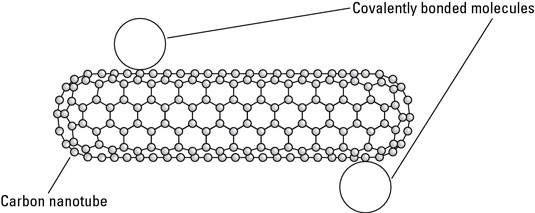
MBBs with three linking groups readily form planar structures because three points define a plane. Graphite, formed from sp2 carbon atoms which bond to three adjacent neighbors, is a planar structure that is quite strong and stiff in two dimensions but which, like paper, is readily folded through a third dimension. Just as paper can be formed into tubes to improve its stiffness, so can graphite be formed into tubes (often called bucky tubes).

MBBs with three linking groups could, like sp2 carbon, form planar structures with good in-plane strength and stiffness, but would be weak and compliant in the third dimension. While this problem could be reduced by forming tubular structures, stiff structures made using this approach would have to be made from many MBBs, as small numbers of MBBs (too few to form tubular structures) would lack stiffness.

MBBs with four linking groups not in a common plane are convenient for building three dimensional structures (much as the four bonds in a tetrahedral sp3 carbon atom allow it to form a stiff, polycyclic three-dimensional diamond lattice).

MBBs with three linking groups can be paired, each member of the pair sacrificing one linking group to form the pair. The pair of MBBs effectively has four linking groups (two available linking groups being provided by each member of the pair). Particularly if the four resulting linking groups are non-planar, the pair can be viewed as a single MBB with four linking groups. In this somewhat roundabout fashion, MBBs with three linking groups can form three dimensional structures much as MBBs with four linking groups.

MBBs with five linking groups can form three dimensional solids. For example, an MBB might have three in-plane linkage groups with inter-linkage-group angles of 120°; and have two out-of-plane linkage groups, both of which are normal to the plane (one linkage group pointing straight up, the other straight down). Such an MBB could form hexagonal sheets by using the three in-plane linkage groups, (each MBB corresponding to a single carbon atom in a sheet of graphite) but would also be able to link together adjacent sheets by using the two out-of-plane linking groups. The unit cell would have hexagonal symmetry.

MBBs with six linking groups can be connected together in a cubic structure, the six linking groups corresponding to the six sides of a cube or rhombohedron. MBBs with six linkage groups can naturally and easily form solid three dimensional structures in the same fashion that cubes or rhomboids can be stacked.

Buckyballs (C60) have now been functionalized with six functional groups (Hutchison et al., 1999; Quin and Rubin, 1999), opening up the possibility of using them as molecular building blocks for the construction of three dimensional structures.

An MBB with six in-plane linkage groups can form a particularly strong planar structure or sheet. The conformation of the sheet would depend only on the length of the inter-MBB links, and not on any ability of the MBB to maintain two linkage groups at some specific angle. As the distance between linked MBBs can often be controlled more effectively (the stretching stiffness of the link can be higher) than the angle between adjacent linkage groups (the bending stiffness is usually lower), this structure can be significantly stiffer in-plane than a planar structure formed from similar MBBs with three linkage groups.

Cubic or hexagonal close packed crystal structures are very stiff, involving 12 linking groups from each MBB. These structures can be described as follows: two very stiff sheets (six linkage groups in-plane) can be laid on top of each other. Each MBB in the upper sheet can be linked to three MBBs in the lower sheet (which form the vertices of a triangle). This arrangement can be repeated with a third, fourth, and more sheets. Six linkage groups connect each MBB to six in-plane neighbors, three linkage groups connect each MBB to three MBBs from the plane below, and three linkage groups connect each MBB to three MBBs from the plane above. The major advantage of this type of MBB is that the stiffness of the whole structure depends only on the stretching stiffness of the links between MBBs and not on the angular stiffness between adjacent linkage groups. This can be useful when the angular stiffness is poor, but the stretching stiffness is good.

MBBs with four linking groups can be paired, each member of the pair sacrificing one linking group to form the pair. The pair of MBBs effectively has six linking groups (three available linking groups being provided by each member of the pair). The pair can be viewed as a single MBB with six linking groups. This again leads naturally to unit cells that are cubic or rhomboid, but with each unit cell comprising two MBBs. This is similar to the primitive unit cell of diamond, which has two carbon atoms.

In summary, MBBs with two linking groups form three dimensional structures only with difficulty and only by using indirect and complex methods. MBBs with three linking groups readily form planar structures, which are strong and stiff in the plane but bend easily, like a sheet of paper, unless rolled into tubular structures to improve stiffness. They can also be used (although somewhat less naturally) to directly form three dimensional solids with a unit cell having four MBBs. MBBs with four linking groups quite naturally form strong, stiff three dimensional solids in which the unit cell is composed of two MBBs (as in diamond). MBBs with five linking groups can readily form strong, stiff three dimensional solids in which the unit cell is composed of six MBBs. MBBs with six linking groups readily form strong, stiff three dimensional solids in which the unit cell is composed of a single MBB. They can also form very stiff sheets if all linkage groups are in-plane, though this arrangement sacrifices stiffness out-of-plane. MBBs with twelve linking groups can form very strong and stiff three dimensional solids.

While MBBs can have any number of linkage groups, MBBs with fewer linkage groups are usually (though not always) more readily synthesized. If we seek an MBB with the least number of linkage groups that can still readily form strong, stiff three dimensional structures, then MBBs with four linkage groups are quite attractive. A high symmetry structure with four linkage groups will have tetrahedral symmetry (with an inter-linkage-group angle of approximately 109°). Much of the discussion in this paper is about specific tetrahedral MBBs.

Self assembled versus positionally assembled MBBs

The design criteria for self assembled MBBs differ in many fundamental respects from the design criteria for positionally assembled MBBs. For example, solubility constraints on positionally assembled MBBs are minimized. MBBs intended for self assembly in solution are usually soluble to permit them to explore differing orientations and positions with respect to each other, eventually settling on an energetically and entropically favored configuration. This solubility constraint is often non-trivial to satisfy and can greatly limit the range of MBBs that can be used.

In contrast, MBBs for positional assembly need not be soluble and do not even need a solvent: they can be used in vacuum. Like bricks, they can be picked up and moved to the desired location whether they are soluble or not.

If two MBBs can bond strongly to each other in two or more different configurations, then the self assembly process will randomly select from among these multiple configurations and produce a random clump of MBBs rather than any specific desired arrangement. For this reason, MBBs for self assembly often use multiple weak bonds, rather than a few strong bonds. Any particular weak bond can be broken by thermal noise. Only when the action of multiple weak bonds is combined does the resulting configuration of MBBs remain stable. Configurations that simultaneously enable multiple weak bonds are relatively rare, and so it is easier to design MBBs with multiple weak bonds that self assemble into a single desired structure.

While the use of strong bonds in self assembly is possible, positional assembly can more readily use MBBs that form a few very strong bonds. Inappropriate interactions between positionally assembled MBBs are prevented by the simple expedient of keeping them away from each other. When two MBBs are brought together, their orientations are controlled to prevent inappropriate bond formation. Thus, selective control over bond formation is achieved through positional control, rather than by designing the MBBs to be selective in bond formation. This approach permits the use of highly reactive MBBs that would be entirely inappropriate for self assembly.

The disadvantage of highly reactive MBBs is that they must be positionally controlled at all times. They cannot be allowed to mix randomly at any time, as this would cause them to rapidly form unusable clumps. While achievable, this imposes a number of constraints that are more difficult to meet with today’s systems.

An alternative approach is to use protecting groups that cover or alter the highly reactive linkage groups. These protecting groups would then be removed when two positionally assembled MBBs were joined. The use of protecting groups is common in chemical synthesis, though the concept of selectively removing a protecting group from a single molecule by using positional control is still novel. Selective photoactivation of molecules within a region comparable in size to the wavelength of light is well known and used commercially. From the perspective of nanotechnology, regions that are hundreds of nanometers in size are very large, making optical approaches rather imprecise when viewed from the perspective of the desired long term objectives.

Positionally assembled MBBs must be held, while self assembled MBBs need not be held. This implies that positionally assembled MBBs must have “handles” by which they can be gripped. While it is possible in some cases to use the linkage groups of the MBB as handles, these linkage groups might well be intended to irreversibly form strong bonds. Because it is essential in positional assembly both to hold the MBB and to let go, such an MBB must be able to form reversible attachments to the positional device. Ideally, this would be done using a variable affinity binding site which has two states: bound and unbound. The tip of the positional device first binds to the MBB. Then it positions the MBB with respect to some workpiece under construction, to which the MBB bonds. Finally, the positional device releases the MBB. Tweezers serve this function: when closed they can grasp an object (high affinity), when open they release the object (low affinity). While there are many other designs for variable affinity binding sites (Merkle, 1997b), tweezers are widely applicable and illustrate the basic concept.

Pragmatically, the greatest advantage of self assembled MBBs is the extensive literature on self assembly and the extensive set of existing experimental techniques that have been used to self assemble some impressively complex structures. Positional assembly at the molecular scale, by contrast, is still in its infancy. For example, the self assembly of DNA into complex molecular structures has made remarkable strides (Seeman, 1994), and has been used to make a truncated octahedron (Zhang, 1994). To quote Seeman and coworkers (Seeman et al., 1997):

There are several advantages to using DNA for nanotechnological constructions. First, the ability to get sticky ends to associate makes DNA the molecule whose intermolecular interactions are the most readily programmed and reliably predicted: Sophisticated docking experiments needed for other systems reduce in DNA to the simple rules that A pairs with T and G pairs with C. In addition to the specificity of interaction, the local structure of the complex at the interface is also known: Sticky ends associate to form B-DNA. A second advantage of DNA is the availability of arbitrary sequences, due to convenient solid support synthesis. The needs of the biotechnology industry have also led to straightforward chemistry to produce modifications, such as biotin groups, fluorescent labels, and linking functions. The recent advent of parallel synthesis is likely to increase the availability of DNA molecules for nanotechnological purposes. DNA-based computing is another area driving the demand for DNA synthetic capabilities. Third, DNA can be manipulated and modified by a large battery of enzymes, including DNA ligase, restriction endonucleases, kinases and exonucleases. In addition, double helical DNA is a stiff polymer in 1-3 turn lengths, it is a stable molecule, and it has an external code that can be read by proteins and nucleic acids. [references omitted from this quote]

The great drawback of self assembly, that it produces weak and compliant structures, can likely be adequately dealt with for transitional systems by careful design and post-modification of the self assembled structure to increase strength and stiffness. While the stiffness of DNA is good in comparison with most other polymers (Hagerman, 1988), it is still poor when compared with bucky tubes, graphite, diamond, silicon, and other “dry” nanotechnology materials.

Abstract properties of tetrahedral MBBs

Tetrahedral positionally assembled MBBs appear to be an attractive alternative, readily forming strong, stiff three dimensional structures while at the same time being simple enough that they can be synthesized. Before considering any specific tetrahedral MBB, we first consider some of their abstract properties.

First and foremost, the linkage groups will have particular properties. Of crucial concern are the conditions under which the links are made, and the extent to which inappropriate links are possible. If a specific functional group, call it R, bonds readily with other functional groups of type R (as is true for radicals), then the MBB cannot be kept in solution without rapidly forming undesired clumps. These limitations can be overcome by the use of protecting groups (or otherwise introducing some barrier to reaction) although this adds the additional requirement that the protecting groups be removed before an MBB is added to a growing workpiece.

A second type of linkage will involve two distinct functional groups, call them A and B. Functional groups of type A will readily bond with functional groups of type B, but A will not bond to A and B will not bond to B. The Diels-Alder reaction (Krummenacker, 1994) is a good illustration of this kind of functional group. The diene and dieneophile (corresponding to functional groups of type A and type B) will bond to each other, but not to themselves. They also bond to little else, and so can be used in most solvents (or in vacuum) and in the presence of impurities. As there are no leaving groups, the reaction itself does not introduce any possibly undesired contaminants.

A second advantage of the A-B functional groups is their increased tolerance of positional uncertainty. Consider two types of MBBs, type A and type B. Type A MBBs have four linkage groups of type A, while type B MBBs have four linkage groups of type B. Type As cannot link with other type As, nor can type Bs link with other type Bs. When type A and type Bs are combined in the diamond (or actuallyzinc-blende or wurtzite (hexagonal)) crystal lattice, they alternate. Each A is surrounded by four Bs, and each B is surrounded by four As.

In both the zinc-blende and wurtzite structures, there are no cycles of length five but many cycles of length six. That is, if we traverse a path from one MBB to another along the links between them, we will never find that we have completed a cycle and returned to the starting MBB without including at least six MBBs along the path. Clearly, a cycle with an odd length (such as five) would imply that either two As were linked or that two Bs were linked. This is forbidden by the nature of the A-B building blocks.

If, however, we were using MBBs of type R, which can readily link to each other, than a path of length five would be possible if the geometry of the MBBs was sufficiently distorted. Such a distortion might occur if the linking groups were insufficiently stiff, and permitted Rs near the edge of the crystal to come into contact with each other. This is exactly what happens on the diamond (100) surface, which forms strained dimers from adjacent carbon atoms which, if they were part of the bulk, would be separated by an additional carbon atom between them.

The use of A-B MBBs eliminates the possibility of odd cycles, and particularly cycles of length five. However, it does not eliminate cycles of length four, which could in principle occur if the geometry were sufficiently strained. As the strain required to achieve a cycle of length four is greater than the strain required to achieve a cycle of length five, R MBBs in a diamond lattice will more readily produce undesired cycles of length five than similar A-B MBBs will produce undesired cycles of length four.

This principle can be extended by introducing more types of functional groups, D, E, F, …. The more types of functional groups, the more strained the geometry must be before an incorrect link can be formed. In the limit, an arbitrary finite structure composed of a fixed number of MBBs arrayed in a regular lattice similar to diamond (or related structures) would have functional groups all of which were distinct and unique. Self assembly of such a structure would occur when the MBBs were mixed, and positional assembly would not be required at all. One method of providing a very large number of distinct types of functional groups is with DNA. There are many short DNA sequences that are selectively sticky, and which would bond only to the appropriate complementary sequence. Experimental work linking gold nanoparticles with DNA suggests this approach is experimentally accessible (Mirkin, 1996).

This illustrates a more general point: self assembly and positional assembly are endpoints on a continuum. As positional accuracy becomes poorer and poorer, “positional” assembly becomes more like self assembly. The techniques used in self assembly to ensure accurate assembly despite positional uncertainty can be gradually introduced into positional assembly as accuracy degrades.

This also illustrates the importance of stiffness in the linkage groups. The stiffer the linkage groups, the less likely that links will be formed where they shouldn’t be. In the limit, sufficiently stiff linkage groups would entirely prevent incorrect structures from forming. Provided the linkage groups have an appropriate orientation, the resulting structures will be unstrained (e.g., tetrahedral sp3 carbon atoms form unstrained bonds in diamond).

Proposals for MBBs

In this section, after reviewing the desirable properties of MBBs, we discuss some specific proposals for MBBs.

MBBs should be stiff, strong, and synthesizable with existing methods. Stiffness and strength are attributes derived from many strong bonds. Polycyclic molecules are usually stronger and stiffer than molecules without cycles (linear or tree structured molecules). Unstrained structures are usually easier to synthesize than strained structures. A good MBB is therefore likely to be polycyclic, with many strong, almost unstrained bonds. Given that bond-bond angles are often 120° (trigonal) or 109° (tetrahedral), we are likely to see hexagonal planar structures (as in graphite), or diamond and related structures. It should therefore come as no surprise that MBBs that resemble bits of graphite with appropriately functionalized edges, or bits of diamond with appropriately functionalized surfaces, are good candidates for MBBs. The diamond lattice in particular can be modified by substitution of carbon by elements from column IV: silicon, germanium, tin, or lead. Edge or surface atoms on the MBB can be chosen from columns III, V or VI, as appropriate (or alternatively the surface atoms can simply be hydrogenated).

Adamantane (hydrogens omitted for clarity)
1,3,5,7-tetraaza-adamantane (methenamine) (hydrogens omitted for clarity)

This line of reasoning leads fairly directly to molecules like adamantane: a stiff tetrahedral molecule which can incorporate heteroatoms and can be readily functionalized. Composed of 10 carbon atoms the Beilstein database (see www.beilstein.com) lists over 20,000 variants, supporting the idea that this family of molecular structures is large, contains many readily synthesized members, and has enough “design space” to provide solutions able to satisfy the multiple constraints imposed on a “good” molecular building block. This conclusion is further supported by (Fort, 1976), who surveyed adamantane chemistry.

A few molecules in this class which have been synthesized include adamantane; 1,3,5,7-tetrasila-adamantane; 1,3,5,7 tetrabora-adamantane (not yet synthesized, though 1-bora-adamantane has been synthesized); 1,3,5,7-tetraaza-adamantane (more commonly known as methenamine, readily synthesized and with a variety of commercial applications (Budavari et al., 1996)); 2,4,6,8,9,10-hexamethyl-2,4,6,8,9,10-hexabora-adamantane; and many others.

Tetramantane (hydrogens omitted for clarity)

Larger bits of diamond that have been synthesized include diamantane (C14H20), triamantane (C18H24), and even tetramantane (C22H28). Pentamantanes (C26H32) and hexamantanes (C30H36) occur naturally in some deep gas deposits (Schoell and Carlson, 1999; Dahl et al., 1999) but are not readily accessible in the laboratory.

Other small stiff structures that might be used as the basis for building blocks include cyclophanes, iceanes (small pieces of “hexagonal diamond,”), buckyballs, buckytubes, alpha helical proteins (Drexler, 1994), and a host of others.

An aside on “bond strength”

Bond “strengths” are typically measured in units of energy. Kcal/mol is common in the chemical literature, though electron volts, joules (more commonly atto joules (10-18 joules) or zepto joules (10-21joules)), Hartrees (atomic units often used in quantum chemistry software) and calories are all used as well. Conversion tables are commonly available. One convenient web page which lists some constants and conversion factors common in nanotechnology (and provides links to other sources) is at http://www.zyvex.com/nanotech/constants.html

In common (non-chemical) usage, “strength” refers to a maximum force, not an energy. Energy and strength are not the same, as the Newtonian equation relating work and force is Work = Force times Distance. Knowing the energy does not tell us the force that must be applied unless we also know the distance over which that force must work. In chemistry, a reasonable approximation to the stretching potential between two bonded atoms is the Morse potential:

U(x) = De[1 – e-b(x-r0)]2

Where U(x) is the potential energy of the system as a function of the separation x between the two bonded atoms, De is the “bond strength” as an energy, e is 2.71828…, r0 is the equilibrium distance (minimum energy distance), and b is a parameter which, along with De, determines the stiffness ks of the bond. As ks is readily determined from the vibrational frequency and the mass of the vibrating atoms, and De (with some adjustment for the zero point vibrational energy) is determined from chemical data about the bond strength, the parameter b can then be determined using the formula (Drexler, 1992):

b = sqrt(ks/ (2 De))

If we pull on the bond with a large enough steady force, it will eventually break. This occurs at a force of b De / 2. Using these equations, and knowing vibrational frequencies, atomic mass, and “bond strength” as an energy, we can compute the actual force required to break a bond. The force required to break a single carbon-carbon bond is ~6 nanonewtons. As the “strength” of the dipolar bond measured as an energy is almost one order of magnitude less, and the stiffness is not substantially less, we would expect that a force of roughly 1 nanonewton would be sufficient to break a dipolar bond.

The use of energies to measure bond strengths is appropriate if we expect that thermal noise is the disruptive force that will break bonds. The time until a bond is thermally disrupted is given by: tbreak = t0eDe/kbT

where kb is Boltzmann’s constant, T is the temperature in Kelvins, and t0 is a constant characteristic of the particular system (on the order of 10-13 for “typical” bonds). As can be seen, bonds with an energy “strength” significantly in excess of thermal noise will not be disrupted by thermal noise for a very long time.

Possible linking groups

As mentioned earlier, polymer chemistry has developed an enormous arsenal of functional groups that can link monomers together. The major drawback from the current perspective is that polymers made from monomers with only two linking groups tend to be floppy — rather than stiff, well defined three dimensional structures. (While proteins can fold into three dimensional structures, the process is indirect). By contrast, tetrahedral MBBs with four functional groups (to take one example) that can link to four other MBBs could be built into very stiff structures. Positional assembly of such MBBs would potentially enable the synthesis of an enormous range of structures. Thus, we wish to increase the number of linking groups per monomer.

How might we link adamantane-based MBBs? (hydrogens omitted for clarity)

How, then, might we link together two adamantane-based MBBs? One possibility which illustrates the concept is the use of dipolar bonds between nitrogen and boron. This is motivated less from any existing common polymer than from the observation that the simplest, stiffest and most direct method of linking two MBBs is to form a bond between two atoms, one atom from each adamantane. While radicals could be used, they suffer from certain drawbacks (clumping during synthesis, for example). The dipolar bond, on the other hand, permits synthesis of the B and N MBBs separately. While much stronger than hydrogen bonds, dipolar bonds are weaker than normal covalent bonds. Their strength can vary substantially, generally in a range from ten to a few tens of kcal/mol.

A central 1,3,5,7 tetrabora-adamantane MBB linked to four surrounding 1,3,5,7-tetraaza-adamantane MBBs.

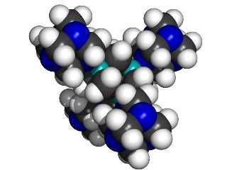
If we use 1,3,5,7 tetrabora-adamantane and 1,3,5,7-tetraaza-adamantane as “B” and “N” building blocks, then each linking atom (N or B) is bonded to three other atoms in its MBB, thus providing a stiff support. The class of structures that can be formed includes the kind of structures typical of (for example) silicon carbide, where alternating silicon and carbon atoms are each bonded to four neighboring atoms of the other type. The B and N type adamantane-based MBBs are, in essence, larger versions of the same concept.

While 1,3,5,7 tetrabora-adamantane has not been synthesized, DFT calculations using a 6-311+G(2d,p) basis set show the molecule is a minima on the potential energy surface (Halls, 1999, private communication). Further, DFT calculations using a somewhat smaller 6-31G(d) basis set show that a dimer composed of an N and a B building block connected by a dipolar bond is also a minima on the potential energy surface with an enthalpy of formation of about 20 kcal/mol (ZPE corrected) (Halls, 1999). While boron with three single bonds is normally planar, it is strained by the tetrahedral nature of the adamantane cage. Stabilization of the boron atoms in the tetrahedral (rather than planar) bonding pattern by suitable electron donor groups (e.g., NH3) should increase the stability of the building-block plus four-donor-groups complex.

Hydrogen bonds

Hydrogen bonds are common in biological systems. They are relatively weak, on the order of 2-5 kcal/mol, but involve straightforward and widely practiced chemistry and can provide reasonable strength when several are combined (Watson et al., 1987). Two carboxcylic acids form a dimer via hydrogen bonds to each other with a ΔH of -14.1 to -16.4 kcal/mol in gas phase (Jones, 1952). If we use adamantane 1,3,5,7 tetracarboxylic acid (four COOH groups at the four trigonal carbon atoms of adamantane) as an MBB, each MBB can readily form eight hydrogen bonds to adjacent MBBs in the crystal if we assume that the MBBs are arranged like the carbon atoms in diamond. However, the resulting crystal structure would have large empty spaces. Experimental determination of the crystal structure (Ermer, 1988) shows five interpentetrating diamondoid lattices, thus effectively filling the large voids that a single diamondoid lattice would create.

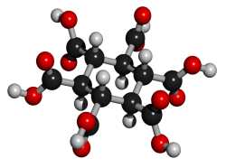
Addendum added January 24, 2002: A theoretical possibility would be cyclohexane-1,3,5/2,4,6-hexacarboxylic acid (see figures at left, the graphic showing the energetically preferred all equatorial isomer). This MBB has six linking groups and each linking group could have two hydrogen bonds. While the all cis isomer — cyclohexane-1,2,3,4,5,6-hexacarboxylic acid with three axial and three equatorial groups — has been synthesized and is available commercially, it does not form an obvious crystal structure in which 12 well aligned hydrogen bonds can form. By contrast, while cyclohexane-1,3,5/2,4,6-hexacarboxylic acid has not been synthesized there is a theoretical crystal structure which forms 12 well aligned hydrogen bonds and has no large voids. Seven such MBB’s arranged in the appropriate structure are shown in the following figure:

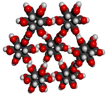
Whether or not this theoretical crystal structure would actually form has not been experimentally determined. No obvious alternative structure would permit good alignment of all 12 hydrogen bonds. The pdb file for a cluster with eight MBB’s is here. There are many readily imaginable variants that have the same or a similar motif.

Addendum added March 15th 2002: “Acid B [all equatorial cyclohexane hexacarboxylic acid] is formed from acid A [all cis cyclohexane hexacarboxylic acid, commercially available] by heating with hydrochloric acid, …” (English translation of German patent by Badische Anilin and Soda-Fabrik Aktiengesellschaft, Convention Application No. 2212369, filed March 15 1972).

A paper that sheds tangential light on the possible crystal structure of “Acid B” is “The crystal structure of mellitic acid, (benzene hexacarboxylic acid)” by S.F. Darlow, Acta Cryst. (1961) 14, pages 159-166. This related molecule forms crystal with a structure as one might expect from the discussion here, differing largely in that it forms layers — a two-dimensional rather than a three-dimensional network of hydrogen bonds.

Tridentate complexes with transition metals

If the six edge atoms in adamantane are replaced with oxygen, then each “face” of the resulting tetrahedron will expose three oxygen atoms, each of which has one of its two lone pairs oriented towards that face. This opens up the possibility of a tridentate complex with an appropriate transition metal. A transition metal which could form a complex with six ligands (octahedral symmetry) could then form two tridentate complexes with the two faces from two neighboring building blocks. Substitutions in the frame of the adamantane cage could alter the spacing and type of the three donating groups (e.g., sulfur instead of oxygen) to permit the tuning of the building block for specific transition metals. This method would orient the other faces of the two building blocks appropriately for a diamond lattice (recall that the C-C-C-C torsion angle in the diamond lattice is n*120° + 60°, i.e., staggered rather than eclipsed; n is an integer).

Six linkage groups using adamantane

Adamantane has four atoms at the vertices of the tetrahedron, and six atoms along the edges of the tetrahedron. These six edge atoms could also be used to link the building blocks together. This would increase the number of links between building blocks (from four to six) thus strengthening the attachment of each building block to the whole. If we just think of carbon-carbon double bonds between adamantanes, the structure would be cubic with a unit cell consisting of 8 adamantane sub-groups. The larger number of linkage groups permitted by this approach might make weaker links more attractive. Hydrogen bonding (Watson, 1987) might prove effective, particularly if small clusters of OH groups could effectively be added despite the obvious steric problems.

Making larger building blocks from smaller ones

Larger building blocks are useful from at least two perspectives: they are easier to manipulate and their larger surface areas provide more sites to bind to other building blocks. While starburst dendrimers let us build large molecular structures from simple building blocks, the resulting structure is specified topologically but can be quite variable structurally.

Using two building blocks that alternate to form a crystal, a somewhat related but more structurally specific process (which we might call starburst crystals) would be to start with a single building block of type A and link it to as many building blocks of type B as possible (typically four or six). This might be done by adding a dilute solution of A to a concentrated solution of B, and then separating the ABnresults, where n corresponds to the number of linkage groups on A, under the assumption that all such linkage groups will be saturated with B building blocks. If the A building block is designated A0, then we might call the A building block surrounded by B building blocks A1.

This process can be repeated, the A1 building block can be mixed into a concentrated solution of A building blocks, adding an additional layer to the growing crystal and producing A2. A2 can be mixed into a concentrated solution of B building blocks, producing A3.

The critical difference between this process and the growth of a starburst dendrimer is that starburst crystalization adds building blocks only at those sites which extend the crystal structure. Thus, a new building block added in the Nth layer might bind to two or even three building blocks from layer N-1. Rather than exponential growth in the number of steps, this process has a growth rate that is cubic in the number of steps and the structure that results can be viewed as that part of a crystal that includes all crystal elements within a certain distance from some center.

If a building block added to layer N links to two building blocks from layer N-1, then it must link to the right two building blocks. If the links between building blocks are sufficiently stiff, this is not a problem. The new building block in layer N can only link appropriate pairs of building blocks from layer N-1. However, if the linkages are too floppy, the new building block might link to an incorrect pair of building blocks from layer N-1, producing an incorrect result. Preventing this requires either control over the geometry of growth (the bonds between building blocks cannot be too floppy) or selective control over linkage formation (different chemistries could be used for the formation of different links, even from the same building block; or linkage groups could be protected and de-protected).

Additive and subtractive synthesis

Given the building blocks and their natural tendency to form a zinc-blende crystal structure (the dipolar bond between two building blocks prefers the staggered rather than the eclipsed form — leading to a structure similar to diamond but with alternating building-block types), the set of structures that can be built include contiguous pieces of crystal with specific building blocks either present or absent. This state of affairs can be reached by one of two alternate routes: start with nothing and add building blocks until the desired structure is complete (additive synthesis), or start with a block which is too large and remove building blocks until the desired structure is reached (subtractive synthesis).

One method of additive synthesis is to add invididual building blocks (rather than groups of building blocks) one at a time. Using positional assembly, this requires a method of grasping and releasing the individual building blocks. As the building blocks already have four sites designed to bind to the complementary building block, these sites could be used to “grip” the building blocks while they were positioned. The tip of the positional device would need to be specifically designed to bind to the building blocks strongly enough to hold them while they were being positioned and oriented, but weakly enough that they could be released when the positional device was withdrawn from the workpiece under construction (or, alternatively, the tip could undergo some change to reduce its binding affinity for the building blocks).

Using substractive synthesis, undesired building blocks could be removed by scraping them away. The major advantage of this approach is that the tip of the positional tool need not bind to the building blocks, and therefore a much wider range of tip structures would be acceptable. Orientation requirements for the tip would also be relaxed. Force applied to a single building block on the surface would break it free from the workpiece. Provided that the bonds holding the building block together were significantly stronger than the bonds between building blocks, whole building blocks would be removed from the workpiece (rather than fragmenting the building blocks).

Subtractive synthesis has another advantage: adding building blocks one by one will on occasion produce situations where the new building block is bound to the workpiece by a single bond (the first building block to be added on a (111) surface, for example). Because it is held by only a single bond, the building block will not be as well bound to the rest of the structure and would have a higher probability of falling off before further building blocks could be added. This is of particular concern when weak bonds are being used between building blocks.

By contrast, substractive synthesis can leave intact all bonds that will be present in the final (desired) structure. If the final structure has been designed so that each building block is held in place by at least two bonds, then at every point during synthesis every building block that will be kept will be held in place by at least two (and often three) bonds. As the probability that a building block will break away from the workpiece is an exponential function of the depth of the potential energy well in which the building block finds itself, and as the depth of this well is doubled when two bonds hold it in place as compared with only a single bond, this difference can be significant.

One of the intriguing aspects of subtractive synthesis is the remarkably wide range of potential building blocks that could be used. Virtually any large, reasonably stiff and reasonably compact organic molecule that remains crystalline at reasonably high temperatures could be used. Adamantane itself, for example, melts at 268°C. (Weast, 1989). Such building blocks would be held together primarily by van der Waals forces, which would increase as the size of the building blocks increased. Precise modification by an SPM in UHV (Ultra High Vacuum) would seem feasible provided the tip was sharp in comparison with the size of the building block. The primary concern would be that building blocks on the surface (rather than in the bulk) might be so weakly bound that they would leave the surface. This could in general be dealt with by lowering the temperature, but a more careful search through the space of possibilities for building blocks that remained bound to the surface at room temperature might prove simpler. It might also be possible to find building blocks that could be selectively removed without the use of UHV, further simplifying the experimental procedure.

What to build?

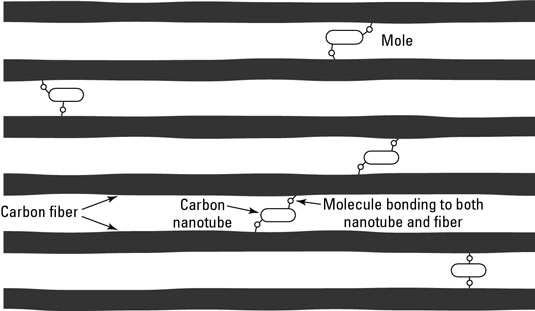
Given a building block, what might we build? While our long term goals must be to build complex molecular machines, in the nearer term we will pursue the construction of key components. One possibility would be a set of molecularly precise tweezers (the use of carbon nanotubes as molecular tweezers has recently been experimentally demonstrated (Kim and Lieber, 1999)). Conceptually simple, a pair of molecularly precise tweezers could be picked up and manipulated by a larger pair of less perfect tweezers. The molecularly precise tweezers would provide well defined surfaces to interact with the part being manipulated.

A second obviously desirable structure would be a joint, which would provide one degree of rotational freedom and essentially no other degrees of freedom. The feasibility of sliding surface joints would depend in large part on the precise nature of the building blocks, but there is in general no problem in designing bearings with sliding surfaces (Merkle, 1993b). If the surfaces are not otherwise attractive to each other (e.g., hydrogen terminated carbon) then well designed bearings should have a small barrier to sliding motion. Bearings made from curved (strained) structures should be feasible at some scale, regardless of the building block, because some degree of strain is always tolerable.

Alternatively, multiple single-linkage-group bearings could be aligned. Two building blocks with intercalating layers could have single rotationally free linkage groups between facing layers. As the layers are molecularly precise, perfect alignment of such single-linkage-group bearings from successive layers would be feasible, thus permitting a molecular bearing of tolerable strength (at least at the molecular scale) to be built.

Finally, a more traditional door-hinge type of joint could be built by using intercalating layers from the two halves of the joint. Rather than attempting to strain the building blocks to provide smooth surfaces, relatively large holes (many building blocks in diameter) could be made which were aligned from layer to layer. A tubular pin (possibly made from strained building blocks, or possibly of some other type, such as buckytubes) could then be inserted through the holes, in the expecation that the smooth surface of the pin would be sufficient to support hinge rotation.

While the use of strained building blocks is feasible, it would also be possible to use building blocks that were “pre-strained.” For example, if a single edge atom in adamantane were changed from C to Si, the resulting building block would no longer be exactly tetrahedrally symmetric. Appropriately “malformed” building blocks could be used on specific crystal surfaces to relieve strain of a particular type. In addition, dislocations could be introduced into the structure. Special building blocks, designed specifically to relieve strain at the core of the specific dislocation, could be used to insure the stability (and feasibility) of the dislocation structure.

Rotary joints are of major importance for positional devices. It is possible to make a Stewart platform using nothing but appropriate rotary joints between otherwise rigid blocks. The design is left as an exercise for the reader — though we note here that each of the six struts in a Stewart platform must support two degrees of freedom at each end, much as a universal joint, and one degree of rotational freedom along the axis of the strut (Merkle, 1997c). Powering movement of the platform by moving the ends of the struts opposite the platform is a separate issue that is not dealt with by this design — though almost any powered one-degree-of-freedom movement of the “free” end of the strut would be sufficient.

Conclusions

The manufacture of molecular machines using positional assembly requires two things: positional devices to do the assembly, and parts to assemble. Molecular building blocks, made from tens to tens of thousands of atoms, provide a rich set of possibilities for parts. Preliminary investigation of this vast space of possibilities suggests that building blocks that have multiple links to other building blocks — at least three, and preferably four or more — will make it easier to positionally assemble strong, stiff three dimensional structures.

Adamantane, C10H16, is a tetrahedrally symmetric stiff hydrocarbon that provides obvious sites for either four, six or more functional groups. Over 20,000 variants of adamantane have been synthesized, providing a rich and well studied set of chemistries.

As positional assembly of molecules has only recently been recognized as a feasible activity, prior research in this area has been limited. No serious barriers to further progress have been identified, quite possibly because serious barriers do not exist. Progress will, however, require substantial further research

M.Tech U-I Atomic and molecular basics

INTRO TO NANO-0

 INTRO TO NANO-3

VSEPR

Hybridization

Intermolecular and intramolecular forces-1

intermolecular-forces-3

SYNTHESIS-3

Unit-I Atomic and Molecular Basics: The scope, The nanoscale systems, Defining nano dimensional materials, Size effects in nano materials, Application and technology development, General methods available for the synthesis of nano dimensional materials.

Particles and Bonds, Chemical bonds in Nano technology, The shapes of molecules, additional aspects of bonding, Molecular geometry: VSEPR Model, Hybridization, Van der Waals interactions, Dipole–Dipole Interactions, Ionic Interactions, Metal bonds, Covalent bonds, Coordinative bonds, Hydrogen bridge bonds and polyvalent bonds.

Nanotechnology is science, engineering, and technology conducted at the nanoscale, which is about 1 to 100 nanometers.

Photo of Richard Feynman
Physicist Richard Feynman, the father of nanotechnology.

Nanoscience and nanotechnology are the study and application of extremely small things and can be used across all the other science fields, such as chemistry, biology, physics, materials science, and engineering.

The ideas and concepts behind nanoscience and nanotechnology started with a talk entitled “There’s Plenty of Room at the Bottom” by physicist Richard Feynman at an American Physical Society meeting at the California Institute of Technology (CalTech) on December 29, 1959, long before the term nanotechnology was used. In his talk, Feynman described a process in which scientists would be able to manipulate and control individual atoms and molecules. Over a decade later, in his explorations of ultraprecision machining, Professor Norio Taniguchi coined the term nanotechnology. It wasn’t until 1981, with the development of the scanning tunneling microscope that could “see” individual atoms, that modern nanotechnology began.

Medieval stained glass window courtesy of NanoBioNet
Medieval stained glass windows are an example of  how nanotechnology was used in the pre-modern era. (Courtesy: NanoBioNet)

It’s hard to imagine just how small nanotechnology is. One nanometer is a billionth of a meter, or 10-9 of a meter. Here are a few illustrative examples:

  • There are 25,400,000 nanometers in an inch
  • A sheet of newspaper is about 100,000 nanometers thick
  • On a comparative scale, if a marble were a nanometer, then one meter would be the size of the Earth

Nanoscience and nanotechnology involve the ability to see and to control individual atoms and molecules. Everything on Earth is made up of atoms—the food we eat, the clothes we wear, the buildings and houses we live in, and our own bodies.

But something as small as an atom is impossible to see with the naked eye. In fact, it’s impossible to see with the microscopes typically used in a high school science classes. The microscopes needed to see things at the nanoscale were invented relatively recently—about 30 years ago.

Once scientists had the right tools, such as the scanning tunneling microscope (STM) and the atomic force microscope (AFM), the age of nanotechnology was born.

Although modern nanoscience and nanotechnology are quite new, nanoscale materials were used for centuries. Alternate-sized gold and silver particles created colors in the stained glass windows of medieval churches hundreds of years ago. The artists back then just didn’t know that the process they used to create these beautiful works of art actually led to changes in the composition of the materials they were working with.

Today’s scientists and engineers are finding a wide variety of ways to deliberately make materials at the nanoscale to take advantage of their enhanced properties such as higher strength, lighter weight, increased control of light spectrum, and greater chemical reactivity than their larger-scale counterparts.

What is Nanotechnology?

 Nanotechnology is the engineering of functional systems at the molecular scale. This covers both current work and concepts that are more advanced.In its original sense, ‘nanotechnology’ refers to the projected ability to construct items from the bottom up, using techniques and tools being developed today to make complete, high performance products.  

With 15,342 atoms, this parallel-shaft speed reducer gear is one of the largest nanomechanical devices ever modeled in atomic detail. LINK

The Meaning of Nanotechnology

When K. Eric Drexler (right) popularized the word ‘nanotechnology’ in the 1980’s, he was talking about building machines on the scale of molecules, a few nanometers wide—motors, robot arms, and even whole computers, far smaller than a cell. Drexler spent the next ten years describing and analyzing these incredible devices, and responding to accusations of science fiction. Meanwhile, mundane technology was developing the ability to build simple structures on a molecular scale. As nanotechnology became an accepted concept, the meaning of the word shifted to encompass the simpler kinds of nanometer-scale technology. The U.S. National Nanotechnology Initiative was created to fund this kind of nanotech: their definition includes anything smaller than 100 nanometers with novel properties.

Much of the work being done today that carries the name ‘nanotechnology’ is not nanotechnology in the original meaning of the word. Nanotechnology, in its traditional sense, means building things from the bottom up, with atomic precision. This theoretical capability was envisioned as early as 1959 by the renowned physicist Richard Feynman.

I want to build a billion tiny factories, models of each other, which are manufacturing simultaneously. . . The principles of physics, as far as I can see, do not speak against the possibility of maneuvering things atom by atom. It is not an attempt to violate any laws; it is something, in principle, that can be done; but in practice, it has not been done because we are too big. — Richard Feynman, Nobel Prize winner in physics

Based on Feynman’s vision of miniature factories using nanomachines to build complex products, advanced nanotechnology (sometimes referred to as molecular manufacturing) will make use of positionally-controlled mechanochemistry guided by molecular machine systems. Formulating a roadmap for development of this kind of nanotechnology is now an objective of a broadly basedtechnology roadmap project led by Battelle (the manager of several U.S. National Laboratories) and the Foresight Nanotech Institute.

Shortly after this envisioned molecular machinery is created, it will result in a manufacturing revolution, probably causing severe disruption. It also has serious economic, social, environmental, and military implications.

Four Generations

Mihail (Mike) Roco of the U.S. National Nanotechnology Initiative has described four generations of nanotechnology development (see chart below). The current era, as Roco depicts it, is that of passive nanostructures, materials designed to perform one task. The second phase, which we are just entering, introduces active nanostructures for multitasking; for example, actuators, drug delivery devices, and sensors. The third generation is expected to begin emerging around 2010 and will feature nanosystems with thousands of interacting components. A few years after that, the first integrated nanosystems, functioning (according to Roco) much like a mammalian cell with hierarchical systems within systems, are expected to be developed.

Some experts may still insist that nanotechnology can refer to measurement or visualization at the scale of 1-100 nanometers, but a consensus seems to be forming around the idea (put forward by the NNI’s Mike Roco) that control and restructuring of matter at the nanoscale is a necessary element. CRN’s definition is a bit more precise than that, but as work progresses through the four generations of nanotechnology leading up to molecular nanosystems, which will include molecular manufacturing, we think it will become increasingly obvious that “engineering of functional systems at the molecular scale” is what nanotech is really all about.

Conflicting Definitions

Unfortunately, conflicting definitions of nanotechnology and blurry distinctions between significantly different fields have complicated the effort to understand the differences and develop sensible, effective policy.

The risks of today’s nanoscale technologies (nanoparticle toxicity, etc.) cannot be treated the same as the risks of longer-term molecular manufacturing (economic disruption, unstable arms race, etc.). It is a mistake to put them together in one basket for policy consideration—each is important to address, but they offer different problems and will require different solutions. As used today, the term nanotechnology usually refers to a broad collection of mostly disconnected fields. Essentially, anything sufficiently small and interesting can be called nanotechnology. Much of it is harmless. For the rest, much of the harm is of familiar and limited quality. But as we will see, molecular manufacturing will bring unfamiliar risks and new classes of problems.

General-Purpose Technology

Nanotechnology is sometimes referred to as a general-purpose technology. That’s because in its advanced form it will have significant impact on almost all industries and all areas of society. It will offer better built, longer lasting, cleaner, safer, and smarter products for the home, for communications, for medicine, for transportation, for agriculture, and for industry in general.

Imagine a medical device that travels through the human body to seek out and destroy small clusters of cancerous cells before they can spread. Or a box no larger than a sugar cube that contains the entire contents of the Library of Congress. Or materials much lighter than steel that possess ten times as much strength. — U.S. National Science Foundation

Dual-Use Technology

Like electricity or computers before it, nanotech will offer greatly improved efficiency in almost every facet of life. But as a general-purpose technology, it will be dual-use, meaning it will have many commercial uses and it also will have many military uses—making far more powerful weapons and tools of surveillance. Thus it represents not only wonderful benefits for humanity, but also grave risks.

A key understanding of nanotechnology is that it offers not just better products, but a vastly improved manufacturing process. A computer can make copies of data files—essentially as many copies as you want at little or no cost. It may be only a matter of time until the building of products becomes as cheap as the copying of files. That’s the real meaning of nanotechnology, and why it is sometimes seen as “the next industrial revolution.”

My own judgment is that the nanotechnology revolution has the potential to change America on a scale equal to, if not greater than, the computer revolution. — U.S. Senator Ron Wyden (D-Ore.)

The power of nanotechnology can be encapsulated in an apparently simple device called a personal nanofactory that may sit on your countertop or desktop. Packed with miniature chemical processors, computing, and robotics, it will produce a wide-range of items quickly, cleanly, and inexpensively, building products directly from blueprints.

Exponential Proliferation

Nanotechnology not only will allow making many high-quality products at very low cost, but it will allow making new nanofactories at the same low cost and at the same rapid speed. This unique (outside of biology, that is) ability to reproduce its own means of production is why nanotech is said to be an exponential technology. It represents a manufacturing system that will be able to make more manufacturing systems—factories that can build factories—rapidly, cheaply, and cleanly. The means of production will be able to reproduce exponentially, so in just a few weeks a few nanofactories conceivably could become billions. It is a revolutionary, transformative, powerful, and potentially very dangerous—or beneficial—technology.

How soon will all this come about? Conservative estimates usually say 20 to 30 years from now, or even much later than that. However, CRN is concerned that it may occur sooner, quite possibly within the next decade. This is because of the rapid progress being made in enabling technologies, such as optics, nanolithography, mechanochemistry and 3D prototyping. If it does arrive that soon, we may not be adequately prepared, and the consequences could be severe.

We believe it’s not too early to begin asking some tough questions and facing the issues:

Who will own the technology?
Will it be heavily restricted, or widely available?
What will it do to the gap between rich and poor?
How can dangerous weapons be controlled, and perilous arms races be prevented?

Many of these questions were first raised over a decade ago, and have not yet been answered. If the questions are not answered with deliberation, answers will evolve independently and will take us by surprise; the surprise is likely to be unpleasant.

It is difficult to say for sure how soon this technology will mature, partly because it’s possible (especially in countries that do not have open societies) that clandestine military or industrial development programs have been going on for years without our knowledge.

We cannot say with certainty that full-scale nanotechnology will not be developed with the next ten years, or even five years. It may take longer than that, but prudence—and possibly our survival—demands that we prepare now for the earliest plausible development scenario.


 Nanoscale

Nanoscale particles are not new in either nature or science. However, the recent leaps in areas such as microscopy have given scientists new tools to understand and take advantage of phenomena that occur naturally when matter is organized at the nanoscale. In essence, these phenomena are based on “quantum effects“ and other simple physical effects such as expanded surface area (more on these below). In addition, the fact that a majority of biological processes occur at the nanoscale gives scientists models and templates to imagine and construct new processes that can enhance their work in medicine, imaging, computing, printing, chemical catalysis, materials synthesis, and many other fields. Nanotechnology is not simply working at ever smaller dimensions; rather, working at the nanoscale enables scientists to utilize the unique physical, chemical, mechanical, and optical properties of materials that naturally occur at that scale.

Nanowires
Computer simulation of electron motions within a nanowire that has a diameter in the nanoscale  range.

When particle sizes of solid matter in the visible scale are compared to what can be seen in a regular optical microscope, there is little difference in the properties of the particles. But when particles are created with dimensions of about 1–100 nanometers (where the particles can be “seen” only with powerful specialized microscopes), the materials’ properties change significantly from those at larger scales. This is the size scale where so-called quantum effects rule the behavior and properties of particles. Properties of materials are size-dependent in this scale range. Thus, when particle size is made to be nanoscale, properties such as melting point, fluorescence, electrical conductivity, magnetic permeability, and chemical reactivity change as a function of the size of the particle.

Nanoscale gold illustrates the unique properties that occur at the nanoscale. Nanoscale gold particles are not the yellow color with which we are familiar; nanoscale gold can appear red or purple. At the nanoscale, the motion of the gold’s electrons is confined. Because this movement is restricted, gold nanoparticles react differently with light compared to larger-scale gold particles. Their size and optical properties can be put to practical use: nanoscale gold particles selectively accumulate in tumors, where they can enable both precise imaging and targeted laser destruction of the tumor by means that avoid harming healthy cells.

A fascinating and powerful result of the quantum effects of the nanoscale is the concept of “tunability” of properties. That is, by changing the size of the particle, a scientist can literally fine-tune a material property of interest (e.g., changing fluorescence color; in turn, the fluorescence color of a particle can be used to identify the particle, and various materials can be “labeled” with fluorescent markers for various purposes). Another potent quantum effect of the nanoscale is known as“tunneling,” which is a phenomenon that enables the scanning tunneling microscope and flash memory for computing.

Over millennia, nature has perfected the art of biology at the nanoscale. Many of the inner workings of cells naturally occur at the nanoscale. For example, hemoglobin, the protein that carries oxygen through the body, is 5.5 nanometers in diameter. A strand of DNA, one of the building blocks of human life, is only about 2 nanometers in diameter.

Drawing on the natural nanoscale of biology, many medical researchers are working on designing tools, treatments, and therapies that are more precise and personalized than conventional ones—and that can be applied earlier in the course of a disease and lead to fewer adverse side-effects. One medical example of nanotechnology is the bio-barcode assay, a relatively low-cost method of detecting disease-specific biomarkers in the blood, even when there are very few of them in a sample. The basic process, which attaches “recognition” particles and DNA “amplifiers” to gold nanoparticles, was originally demonstrated at Northwestern University for a prostate cancer biomarker following prostatectomy. The bio-barcode assay has proven to be considerably more sensitive than conventional assays for the same target biomarkers, and it can be adapted to detect almost any molecular target.i

Growing understanding of nanoscale biomolecular structures is impacting other fields than medicine. Some scientists are looking at ways to use nanoscale biological principles of molecular self-assembly, self-organization, and quantum mechanics to create novel computing platforms. Other researchers have discovered that in photosynthesis, the energy that plants harvest from sunlight is nearly instantly transferred to plant “reaction centers” by quantum mechanical processes with nearly 100% efficiency (little energy wasted as heat). They are investigating photosynthesis as a model for “green energy” nanosystems for inexpensive production and storage of nonpolluting solar power.ii

Nanoscale materials have far larger surface areas than similar masses of larger-scale materials. As surface area per mass of a material increases, a greater amount of the material can come into contact with surrounding materials, thus affecting reactivity.

A simple thought experiment shows why nanoparticles have phenomenally high surface areas. A solid cube of a material 1 cm on a side has 6 square centimeters of surface area, about equal to one side of half a stick of gum. But if that volume of 1 cubic centimeter were filled with cubes 1 mm on a side, that would be 1,000 millimeter-sized cubes (10 x 10 x 10), each one of which has a surface area of 6 square millimeters, for a total surface area of 60 square centimeters—about the same as one side of two-thirds of a 3” x 5” note card. When the 1 cubic centimeter is filled with micrometer-sized cubes—a trillion (1012) of them, each with a surface area of 6 square micrometers—the total surface area amounts to 6 square meters, or about the area of the main bathroom in an average house. And when that single cubic centimeter of volume is filled with 1-nanometer-sized cubes—1021 of them, each with an area of 6 square nanometers—their total surface area comes to 6,000 square meters. In other words, a single cubic centimeter of cubic nanoparticles has a total surface area one-third larger than a football field!

Nanocubes
Illustration demonstrating the effect of the increased surface area provided by nanostructured materials

One benefit of greater surface area—and improved reactivity—in nanostructured materials is that they have helped create better catalysts. As a result, catalysis by engineered nanostructured materials already impacts about one-third of the huge U.S.—and global—catalyst markets, affecting billions of dollars of revenue in the oil and chemical industries.iii An everyday example of catalysis is the catalytic converter in a car, which reduces the toxicity of the engine’s fumes. Nanoengineered batteries, fuel cells, and catalysts can potentially use enhanced reactivity at the nanoscale to produce cleaner, safer, and more affordable modes of producing and storing energy.

Large surface area also makes nanostructured membranes and materials ideal candidates for water treatment and desalination (e.g., see “Self-Assembled, Nanostructured Carbon for Energy Storage and Water Treatment” in our database,NNI Accomplishments Archive), among other uses. It also helps support “functionalization” of nanoscale material surfaces (adding particles for specific purposes), for applications ranging from drug delivery to clothing insulation.

Synthesis of Nanomaterials

It is classified as bottom-up manufacturing which involves building up of the atom or molecular constituents as against the top method which involves making smaller and smaller structures through etching from the bulk material as exemplified by the semiconductor industry.

Gas Condensation

Gas condensation was the first technique used to synthesize nanocrystalline metals and alloys. In this technique, a metallic or inorganic material is vaporized using thermal evaporation sources such as a Joule heated refractory crucibles, electron beam evaporation devices, in an atmosphere of 1-50 m bar. In gas evaporation, a high residual gas pressure causes the formation of ultra fine particles (100 nm) by gas phase collision. The ultrafiine particles are formed by collision of evaporated atoms with residual gas molecules. Gas pressures greater than 3 mPa (10 torr) are required.  Vaporization sources may be resistive heating, high energy electron beams, low energy electron beam and inducting heating. Clusters form in the vicinity of the source by homogenous nucleation in the gas phase grew by incorporation by atoms in the gas phase. It comprises of a ultra high vacuum (UHV) system fitted evaporation source, a cluster collection device of liquid nitrogen filled cold finger scrapper assembly and compaction device. During heating, atoms condense in the supersaturation zone close to Joule heating device. The nanoparticles are removed by scrapper in the form of a metallic plate. Evaporation is to be done from W, Ta or Mo refractory metal crucibles. If the metals react with crucibles, electron beam evaporation technique is to be used. The method is extremely slow. The method suffers from limitations such as a source-precursor incompatibility, temperature ranges and dissimilar evaporation rates in an alloy. Alternative sources have been developed over the years. For instance, Fe is evaporated into an inert gas atmosphere (He). Through collision with the atoms the evaporated Fe atoms loose kinetic energy and condense in the form of small crystallite crystals, which accumulate as a loose powder. Sputtering or laser evaporation may be used instead of thermal evaporation. Sputtering is a non-thermal process in which surface atoms are physically ejected from the surface by momentum transfer from an energetic bombarding species of atomic/molecular size. Typical sputtering uses a glow discharge or ion beam. Interaction events which occur at and near the target surface during the sputtering process in magnetron sputtering has advantage over diode and triode sputtering. In magnetron sputtering, most of the plasma is confined to the near target region. Other alternate energy sources which have been successfully used to produce clusters or ultra fine particles are sputtering electron beam heating and plasma methods. Sputtering has been used in low pressure environment to produce a variety of clusters including Ag, Fe and Si.

Vacuum Deposition and Vaporization

Before proceeding to the other methods, it is important to understand the terms vacuum deposition and vaporization or vacuum evaporation. In vacuum deposition process, elements, alloys or compounds are vaporized and deposited in a vacuum . The vaporization source is the one that vaporizes materials by thermal processes. The process is carried out at pressure of less than 0.1 Pa (1 m Torr) and in vacuum levels of 10 to 0.1 MPa. The substrate temperature ranges from ambient to 500°C. The saturation or equilibrium vapor pressure of a material is defined as the vapor pressure of the material in equilibrium with the solid or liquid surface. For vacuum deposition, a reasonable deposition rate can be obtained if the vaporization rate is fairly high. A useful deposition rate is obtained at a vapor pressure of 1.3 Pa (0.01 Torr).

Vapor phase nucleation can occur in dense vapor cloud by multibody collisions, The atoms are passed through a gas to provide necessary collision and cooling for nucleation. These particles are in the range of 1 to 100 nm and are called ultra fine particles or clusters. The advantages associated with vacuum deposition process are high deposition rates and economy. However, the deposition of many compounds is difficult. Nanoparticles produced from a supersaturated vapor are usually longer than the cluster.

Chemical Vapor Deposition (CVD) and Chemical Vapor Condensation (CVC)

CVD is a well known process in which a solid is deposited on a heated surface via a chemical reaction from the vapor or gas phase. CVC reaction requires activation energy to proceed. This energy can be provided by several methods. In thermal CVD the reaction is activated by a high temperature above 900oC. A typical apparatus comprises of gas supply system, deposition chamber and an exhaust system. In plasma CVD, the reaction is activated by plasma at temperatures between 300 and 700°C. In laser CVD, pyrolysis occurs when laser thermal energy heats an absorbing substrate. In photo-laser CVD, the chemical reaction is induced by ultra violet radiation which has sufficient photon energy, to break the chemical bond in the reactant molecules. In this process, the reaction is photon activated and deposition occurs at room temperature. Nano composite powders have been prepared by CVD. SiC/Si3N composite powder was prepared using SiH4, CH4, WF6 and H2 as a source of gas at 1400°C. Another process called chemical vapor condensation (CVC) was developed in Germany in 1994. It involves pyrolysis of vapors of metal organic precursors in a reduced pressure atmosphere. Particles of ZrO2, Y2O3 and nanowhiskers have been produced by CVC method. A metalorganic precursor is introduced in the hot zone of the reactor using mass flow controller. For instance, hexamethyldisilazane (CH3)3 Si NHSi (CH3)3 was used to produce SiCxNyOz powder by CVC technique. The reactor allows synthesis of mixtures of nanoparticles of two phases or doped nanoparticles by supplying two precursors at the front end of reactor and coated nanoparticles, n-ZrO2, coated with n-Al2O3 by supplying a second precursor in a second stage of reactor. The process yields quantities in excess of 20 g/hr. The yield can be further improved by enlarging the diameter of hot wall reactor and mass of fluid through the reactor. Typical nanocrystalline materials which have been synthesized are shown in Table 1.

Table 1. Typical nanocrystalline materials synthesized by the CVC method

Precursor Product Powder Phase
as prepared
Average Particle size (nm) Surface Area (m2/g)
(CH3) 3SiNHSi(CH3) 3 SiCxNyOz Amorphous 4 377
Si(CH3)4 SiC β-phase 9 201
Al[2-OC4H9]3 Al2O3 Amorphous 3.5 449
Ti[I-OC3H7]4 TiO2 Anatase 8 193
Si[OC2H5]4 SiO2 Amorphous 6 432
Zr[3-OC4H9]4 ZrO2 Monoclinic 7 134

Mechanical Attrition

Unlike many of the methods mentioned above, mechanical attrition produces its nanostructures not by cluster assembly but by the structural decomposition of coarser grained structures as a result of plastic deformation. Elemental powders of Al and β-SiC were prepared in a high energy ball mill. More recently, ceramic/ceramic nanocomposite WC-14% MgO material has been fabricated. The ball milling and rod milling techniques belong to the mechanical alloying process which has received much attention as a powerful tool for the fabrication of several advanced materials. Mechanical alloying is a unique process, which can be carried out at room temperature. The process can be performed on both high energy mills, centrifugal type mill and vibratory type mill, and low energy tumbling mill.

Examples of High Energy Mills

High energy mills include:

  • Attrition Ball Mill
  • Planetary Ball Mill
  • Vibrating Ball Mill
  • Low Energy Tumbling Mill
  • High Energy Ball Mill

Attrition Ball Mill

The milling procedure takes place by a stirring action of a agitator which has a vertical rotator central shaft with horizontal arms (impellers). The rotation speed was later increased to 500 rpm. Also, the milling temperature was in greater control.

Planetary Ball Mill

Centrifugal forces are caused by rotation of the supporting disc and autonomous turning of the vial. The milling media and charge powder alternatively roll on the inner wall of the vial and are thrown off across the bowl at high speed (360 rpm).

Vibrating Ball Mill

It is used mainly for production of amorphous alloys. The changes of powder and milling tools are agitated in the perpendicular direction at very high speed (1200 rpm).

Low Energy Tumbling Mill

They have been used for successful preparation of mechanically alloyed powder. They are simple to operate with low operation costs. A laboratory scale rod mill was used to prepare homogenous amorphous Al30Ta70 powder by using S.S. cylinder rods. Single-phase amorphous powder of AlxTm100-x with low iron concentration can be formed by this technique.

High Energy Ball Mill

High-energy ball milling is an already established technology, however, it has been considered dirty because of contamination problems with iron. However, the use of tungsten carbide component and inert atmosphere and /or high vacuum processes has reduced impurity levels to within acceptable limits. Common drawbacks include low surface, highly poly disperse size distribution, and partially amorphous state of the powder. These powders are highly reactive with oxygen, hydrogen and nitrogen. Mechanical alloying leads to the fabrication of alloys, which cannot be produced by conventional techniques. It would not be possible to produce an alloy of Al-Ta, because of the difference in melting points of Al (933 K) and Ta (3293 K) by any conventional process. However, it can be fabricated by mechanical alloying using ball milling process.

Other Processes

Several other processes such as hydrodynamic cavitation micro emulsion and sonochemical processing techniques have also been used. In cavitation process nanoparticles are generated through creation and release of gas bubbles inside the sol-gel solution. By pressurizing in super critical drying chamber and exposing to cavitational disturbances and high temperature heating, the sol-gel is mixed. Te erupted hydrodynamic bubbles cause the nucleation, growth and quenching of nanoparticles. Particle size can be controlled by adjusting pressure and solution retention times.

Sol-Gel Techniques

In addition to techniques mentioned above, the sol-gel processing techniques have also been extensively used. Colloidal particles are much larger than normal molecules or nanoparticles. However, upon mixing with a liquid colloids appear bulky whereas the nanosized molecules always look clear. It involves the evolution of networks through the formation of colloidal suspension (sol) and gelatin to form a network in continuous liquid phase (gel). The precursor for synthesizing these colloids consists of ions of metal alkoxides and aloxysilanes. The most widely used are tetramethoxysilane (TMOS), and tetraethoxysilanes (TEOS) which form silica gels. Alkoxides are immiscible in water. They are organo metallic precursors for silica, aluminum, titanium, zirconium and many others. Mutual solvent alcohol is used. The sol gel process involves initially a homogeneous solution of one or more selected alkoxides. These are organic precursors for silica, alumina, titania, zirconia, among others. A catalyst is used to start reaction and control pH. Sol-gel formation occurs in four stages.

  • Hydrolysis
  • Condensation
  • Growth of particles
  • Agglomeration of particles

Hydrolysis

During hydrolysis, addition of water results in the replacement of [OR] group with [OH-] group. Hydrolysis occurs by attack of oxygen on silicon atoms in silica gel. Hydrolysis can be accelerated by adding a catalyst such as HCl and NH3. Hydrolysis continues until all alkoxy groups are replaced by hydroxyl groups. Subsequent condensation involving silanol group (Si-OH) produced siloxane bonds (Si-O-Si) and alcohol and water. Hydrolysis occurs by attack of oxygen contained in the water on the silicon atom.

Condensation

Polymerization to form siloxane bond occurs by either a water producing or alcohol producing condensation reaction. The end result of condensation products is the formation of monomer, dimer, cyclic tetramer, and high order rings. The rate of hydrolysis is affected by pH, reagent concentration and H2O/Si molar ratio (in case of silica gels). Also ageing and drying are important. By control of these factors, it is possible to vary the structure and properties of sol-gel derived inorganic networks.

Growth and Agglomeration

As the number of siloxane bonds increase, the molecules aggregate in the solution, where they form a network, a gel is formed upon drying. The water and alcohol are driven off and the network shrinks. At values of pH of greater then 7, and H2O/Si value ranging from 7 to 5. Spherical nano-particles are formed. Polymerization to form siloxane bonds by either an alcohol producing or water producing condensate occurs.

2 HOSi (OR)3 → (OR)3 Si O Si (OR)3 + H2O

or

2 HOSi (OR) 3 → (OR)2OH Si O Si (OR)3 + H2O

Above pH of 7, Silica is more soluble and silica particles grow in size. Growth stops when the difference in solubility between the smallest and largest particles becomes indistinguishable. Larger particles are formed at higher temperatures. Zirconium and Yttrium gels can be similarly produced.

Despite improvements in both chemical and physical methods of synthesis, there remain some problems and limitations. Laser vaporization technique has offered several advantages over other heating techniques. A high energy pulsed laser with an intensity flux of 106 – 107 W/cm2 is forced on target material. The plasma causes high vaporization and high temperature (10,000°C). Typical yields are 1014-1015 atoms from the surface area of 0.01 cm2 in a 10-8 s pulse. Thus a high density of vapor is produced in a very short time (10-8 s), which is useful for direct deposition of particles.

Electrodeposition

Nanostructured materials can also be produced by electrodeposition. These films are mechanically strong, uniform and strong. Substantial progress has been made in nanostructured coatings applied either by DVD or CVD. Many other non-conventional processes such as hypersonic plasma particle deposition (HPPD) have been used to synthesize and deposit nanoparticles. The significant potential of nanomaterial synthesis and their applications is virtually unexplored. They offer numerous challenges to overcome. Understanding more of synthesis would help in designing better materials. It has been shown that certain properties of nanostructured deposits such as hardness, wear resistance and electrical resistivity are strongly affected by grain size. A combination of increased hardness and wear resistance results in a superior coating performance.

CHEMICAL BOND IN NANOTECHNOLOGY

The properties of nanoparticles can be customized for use in a particular nanotechnology application by bonding molecules to the nanoparticles in a process called functionalization. In addition, the capability to build nanocomposites, materials formed by integrating nanoparticles into the structure of a bulk material, makes it possible to create new materials that offer a range of new possibilities.

Fundamentals of nanotech functionalization

When an atom is attached to another atom, the attachment is called a chemical bond. Functionalization is a process that involves attaching atoms or molecules to the surface of a nanoparticle with a chemical bond to change the properties of that nanoparticle.

The bond used in functionalization can be either a covalent bond or a van der Waals bond. Covalent bonding, in which electrons are shared between the atoms involves an atom on the nanoparticle sharing electrons with an atom on the molecule, creating a very strong bond.

In a van der Waals bond, electrostatic attraction occurs (negative and positive charges on the molecules and nanoparticles attract each other). A positively charged region of the molecule or nanoparticle and a negatively charged region of the molecule or nanoparticle form a bond. The van der Waals bond is not as strong as a covalent bond, but it also does not weaken the structures being bonded, as covalent bonds do.

Functionalizing a carbon nanotube by covalently bonding molecules to it.

Functionalizing a carbon nanotube by covalently bonding molecules to it.

For example, if you are bonding molecules to carbon nanotubes, a covalent bond might weaken the nanotube while a van der Waals bond would not. Therefore, although covalent bonds are used more often for functionalization, van der Waals bonding is sometimes useful. One such use is functionalizing a carbon nanotube by bonding a molecule to the nanotube using van der Waals force.

Functionalizing a carbon nanotube by attaching a molecule to it using van der Waals bonding.

Functionalizing a carbon nanotube by attaching a molecule to it using van der Waals bonding.

Functionalization is used to prepare nanoparticles for many uses, for example:

  • Making sensor elements that can be used to detect very low levels of chemical or biological molecules or for the diagnosis of a blood sample.

  • Bonding nanoparticles to fibers or polymers to form lightweight, high-strength composites.

  • Making nanoparticles that can bond to biological molecules present on the surface of diseased cells to produce targeted drug delivery agents.

  • Making nanoparticles that are attracted to prepared attachment sites, such as surfaces containing certain types of atoms (sulfur is attracted to gold, for example) for self-aligned assembly.

Make nanocomposites from functionalized nanoparticles

When you include functionalized nanoparticles in a composite material, those nanoparticles can form covalent bonds with the primary material used in the composite. For example, functionalized nanotubes can bond with polymers to produce a stronger plastic. In a carbon fiber composite, functionalized nanotubes bond with the carbon fibers to create a stronger structure.

Functionalized nanotubes forming a strong bond with carbon fibers.

Functionalized nanotubes forming a strong bond with carbon fibers.

Nanocomposites are being used in several applications:

  • A variety of nanoparticles such as buckyballs, nanotubes, and silica nanoparticles are being used with various fibers to form nanocomposites used in sports equipment such as tennis racquets to improve their strength or stiffness while keeping them lightweight.

  • Nanocomposites using carbon nanotubes and polymers are being developed to make lighter-weight spacecraft.

  • Nanocomposites using carbon nanotubes in an epoxy are being used to make windmill blades longer, enabling the windmill to generate more electricity.

  • Nanoparticles of clay are used in plastic composites to reduce the leakage of carbon dioxide from plastic bottles, improving the shelf life of carbonated beverages.

  • Composites of nanoparticles and polymers are being developed to produce lightweight, strong plastics to replace metals in cars.

    VSEPR  MODEL

  • Predicting the Shapes of Molecules

    There is no direct relationship between the formula of a compound and the shape of its molecules. The shapes of these molecules can be predicted from their Lewis structures, however, with a model developed about 30 years ago, known as the valence-shell electron-pair repulsion (VSEPR) theory.

    The VSEPR theory assumes that each atom in a molecule will achieve a geometry that minimizes the repulsion between electrons in the valence shell of that atom. The five compounds shown in the figure below can be used to demonstrate how the VSEPR theory can be applied to simple molecules.

    Table of Geometries

    There are only two places in the valence shell of the central atom in BeF2 where electrons can be found. Repulsion between these pairs of electrons can be minimized by arranging them so that they point in opposite directions. Thus, the VSEPR theory predicts that BeF2 should be a linear molecule, with a 180o angle between the two Be-F bonds.

    Structure

    There are three places on the central atom in boron trifluoride (BF3) where valence electrons can be found. Repulsion between these electrons can be minimized by arranging them toward the corners of an equilateral triangle. The VSEPR theory therefore predicts a trigonal planar geometry for the BF3 molecule, with a F-B-F bond angle of 120o.

    Structure

    BeF2 and BF3 are both two-dimensional molecules, in which the atoms lie in the same plane. If we place the same restriction on methane (CH4), we would get a square-planar geometry in which the H-C-H bond angle is 90o. If we let this system expand into three dimensions, however, we end up with a tetrahedral molecule in which the H-C-H bond angle is 109o28′.

    Structure

    Repulsion between the five pairs of valence electrons on the phosphorus atom in PF5 can be minimized by distributing these electrons toward the corners of a trigonal bipyramid. Three of the positions in a trigonal bipyramid are labeled equatorial because they lie along the equator of the molecule. The other two are axial because they lie along an axis perpendicular to the equatorial plane. The angle between the three equatorial positions is 120o, while the angle between an axial and an equatorial position is 90o.

    Structure

    There are six places on the central atom in SF6 where valence electrons can be found. The repulsion between these electrons can be minimized by distributing them toward the corners of an octahedron. The term octahedron literally means “eight sides,” but it is the six corners, or vertices, that interest us. To imagine the geometry of an SF6 molecule, locate fluorine atoms on opposite sides of the sulfur atom along the X, Y, and Z axes of an XYZ coordinate system.

    Structure


    Incorporating Double and Triple Bonds Into the VSEPR Theory

    Compounds that contain double and triple bonds raise an important point: The geometry around an atom is determined by the number of places in the valence shell of an atom where electrons can be found, not the number of pairs of valence electrons. Consider the Lewis structures of carbon dioxide (CO2) and the carbonate (CO32-) ion, for example.

    Structures

    There are four pairs of bonding electrons on the carbon atom in CO2, but only two places where these electrons can be found. (There are electrons in the C=O double bond on the left and electrons in the double bond on the right.) The force of repulsion between these electrons is minimized when the two C=O double bonds are placed on opposite sides of the carbon atom. The VSEPR theory therefore predicts that CO2 will be a linear molecule, just like BeF2, with a bond angle of 180o.

    The Lewis structure of the carbonate ion also suggests a total of four pairs of valence electrons on the central atom. But these electrons are concentrated in three places: The two C-O single bonds and the C=O double bond. Repulsions between these electrons are minimized when the three oxygen atoms are arranged toward the corners of an equilateral triangle. The CO32- ion should therefore have a trigonal-planar geometry, just like BF3, with a 120o bond angle.


    The Role of Nonbonding Electrons in the VSEPR Theory

    The valence electrons on the central atom in both NH3 and H2O should be distributed toward the corners of a tetrahedron, as shown in the figure below. Our goal, however, isn’t predicting the distribution of valence electrons. It is to use this distribution of electrons to predict the shape of the molecule. Until now, the two have been the same. Once we include nonbonding electrons, that is no longer true.

    Diagram

    The VSEPR theory predicts that the valence electrons on the central atoms in ammonia and water will point toward the corners of a tetrahedron. Because we can’t locate the nonbonding electrons with any precision, this prediction can’t be tested directly. But the results of the VSEPR theory can be used to predict the positions of the nuclei in these molecules, which can be tested experimentally. If we focus on the positions of the nuclei in ammonia, we predict that the NH3 molecule should have a shape best described as trigonal pyramidal, with the nitrogen at the top of the pyramid. Water, on the other hand, should have a shape that can be described as bent, or angular. Both of these predictions have been shown to be correct, which reinforces our faith in the VSEPR theory.

    When we extend the VSEPR theory to molecules in which the electrons are distributed toward the corners of a trigonal bipyramid, we run into the question of whether nonbonding electrons should be placed in equatorial or axial positions. Experimentally we find that nonbonding electrons usually occupy equatorial positions in a trigonal bipyramid.

    To understand why, we have to recognize that nonbonding electrons take up more space than bonding electrons. Nonbonding electrons need to be close to only one nucleus, and there is a considerable amount of space in which nonbonding electrons can reside and still be near the nucleus of the atom. Bonding electrons, however, must be simultaneously close to two nuclei, and only a small region of space between the nuclei satisfies this restriction.

    Because they occupy more space, the force of repulsion between pairs of nonbonding electrons is relatively large. The force of repulsion between a pair of nonbonding electrons and a pair of bonding electrons is somewhat smaller, and the repulsion between pairs of bonding electrons is even smaller.

    The figure below can help us understand why nonbonding electrons are placed in equatorial positions in a trigonal bipyramid.

    Diagram

    If the nonbonding electrons in SF4 are placed in an axial position, they will be relatively close (90o) to three pairs of bonding electrons. But if the nonbonding electrons are placed in an equatorial position, they will be 90o away from only two pairs of bonding electrons. As a result, the repulsion between nonbonding and bonding electrons is minimized if the nonbonding electrons are placed in an equatorial position in SF4.

    The results of applying the VSEPR theory to SF4, ClF3, and the I3 ion are shown in the figure below.

    Diagram

    When the nonbonding pair of electrons on the sulfur atom in SF4 is placed in an equatorial position, the molecule can be best described as having a see-saw or teeter-totter shape. Repulsion between valence electrons on the chlorine atom in ClF3 can be minimized by placing both pairs of nonbonding electrons in equatorial positions in a trigonal bipyramid. When this is done, we get a geometry that can be described as T-shaped. The Lewis structure of the triiodide (I3) ion suggests a trigonal bipyramidal distribution of valence electrons on the central atom. When the three pairs of nonbonding electrons on this atom are placed in equatorial positions, we get a linear molecule.

    Molecular geometries based on an octahedral distribution of valence electrons are easier to predict because the corners of an octahedron are all identical.


Intermolecular Interactions in the Gas Phase


Interactions between two or more molecules are called intermolecular interactions, while the interactions between the atoms within a molecule are called intramolecular interactions.  Intermolecular interactions occur between all types of molecules or ions in all states of matter.  They range from the strong, long-distance electrical attractions and repulsions between ions to the relatively weak dispersion forces which have not yet been completely explained.  The various types of interactions are classified as (in order of decreasing strength of the interactions):

ion – ion
ion – dipole
dipole – dipole
ion – induced dipole
dipole – induced dipole
dispersion forces

Without these interactions, the condensed forms of matter (liquids and solids) would not exist except at extremely low temperatures.  We will explore these various forces and interactions in the gas phase to understand why some materials vaporize at very low temperatures, and others persist as solids or liquids to extremely high temperatures.

Ion – Ion Interactions

The interactions between ions (ion – ion interactions) are the easiest to understand: like charges repel each other and opposite charges attract.  These Coulombic forces operate over relatively long distances in the gas phase.  The force depends on the product of the charges (Z1, Z2) divided by the square of the distance of separation (d2):

 F = – Z1Z2/d2

 Two oppositely-charged particles flying about in a vacuum will be attracted toward each other, and the force becomes stronger and stronger as they approach until eventually they will stick together and a considerable amount of energy will be required to separate them.  They form an ion-pair, a new particle which has a positively-charged area and a negatively-charged area.  There are fairly strong interactions between these ion pairs and free ions, so that these the clusters tend to grow, and they will eventually fall out of the gas phase as a liquid or solid (depending on the temperature).

Ion – Ion Interactions in the Gas Phase

top


Dipole Moment

Let’s go back to that first ion pair which was formed when the positive ion and the negative ion came together.  If the electronegativities of the elements are sufficiently different (like an alkali metal and a halide), the charges on the paired ions will not change appreciably – there will be a full electron charge on the blue ion and a full positive charge on the red ion.  The bond formed by the attraction of these opposite charges is called an ionic bond.  If the difference in electronegativity is not so great, however, there will be some degree of sharing of the electrons between the two atoms.  The result is the same whether two ions come together or two atoms come together:

Polar Molecule

The combination of atoms or ions is no longer a pair of ions, but rather a polar molecule which has a measureable dipole moment.  The dipole moment (D) is defined as if there were a positive (+q) and a negative (-q) charge separated by a distance (r):
                        D = qr
If there is no difference in electronegativity between the atoms (as in a diatomic molecule such as O2 or F2) there is no difference in charge and no dipole moment.  The bond is called acovalent bond, the molecule has no dipole moment, and the molecule is said to be non-polar. Bonds between different atoms have different degrees of ionicity depending on the difference in the electronegativities of the atoms.  The degree of ionicity may range from zero (for a covalent bond between two atoms with the same electronegativity) to one (for an ionic bond in which one atom has the full charge of an electron and the other atom has the opposite charge).  In some cases, two or more partially ionic bonds arranged symmetrically around a central atom may mutually cancel each other’s polarity, resulting in a non-polar molecule.  An example of this is seen in the carbon tetrachloride (CCl4) molecule.  There is a substantial difference between the electronegativities of carbon (2.55) and chlorine (3.16), but the four chlorine atoms are arranged symmetrically about the carbon atom in atetrahedral configuration, and the molecule has zero dipole momentSaturated hydrocarbons (CnHn+2) are non-polar molecules because of the small difference in the electronegativities of carbon and hydrogen plus the near symmetry about each carbon atom.

Non-polar Molecule

top

Polar molecules can interact with ions:

Ion – Dipole Interactions

or with other polar molecules:

Dipole – Dipole Interactions

top


The charges on ions and the charge separation in polar molecules explain the fairly strong interactions between them, with very strong ion – ion interactions, weaker ion – dipole interactions, and considerably weaker dipole – dipole interactions.  Even in a non-polar molecule, however, the valence electrons are moving around and there will occasionally be instances when more are on one side of the molecule than on the other.  This gives rise to fluctuating or instantaneous dipoles:

Fluctuating Dipole in a Non-polar Molecule

These instantaneous dipoles may be induced and stabilized as an ion or a polar molecule approaches the non-polar molecule.

Ion – Induced Dipole Interaction

Dipole – Induced Dipole Interaction

top


Dispersion Forces

Interactions between ions, dipoles, and induced dipoles account for many properties of molecules – deviations from ideal gas behavior in the vapor state, and the condensation of gases to the liquid or solid states.  In general, stronger interactions allow the solid and liquid states to persist to higher temperatures.  However, non-polar molecules show similar behavior, indicating that there are some types of intermolecular interactions that cannot be attributed to simple electrical attractions.  These interactions are generally called dispersion forces.  Electrical forces operate when the molecules are several molecular diameters apart, and become stronger as the molecules or ions approach each other.  Dispersion forces are very weak until the molecules or ions are almost touching each other, as in the liquid state.  These forces appear to increase with the number of “contact points” with other molecules, so that long non-polar molecules such as n-octane (C8H18) may have stronger intermolecular interactions than very polar molecules such as water (H2O), and the boiling point of n-octane is actually higher than that of water.

Dispersion Forces


It is possible that these forces arise from the fluctuating dipole of one molecule inducing an opposing dipole in the other molecule, giving an electrical attraction.  It is also possible that these interactions are due to some sharing of electrons between the molecules in “intermolecular orbitals“, similar to the “molecular orbitals” in which electrons from two atoms are shared to form a chemical bond.  These dispersion forces are assumed to exist between all molecules and/or ions when they are sufficiently close to each other.  The stronger farther-reaching electrical forces from ions and dipoles are considered to operate in addition to these forces.

Chemical Bond Types

Overview

Ionic Bonds

An ionic bond is formed by the attraction of oppositely charged atoms or groups of atoms. When an atom (or group of atoms) gains or loses one or more electrons, it forms an ion. Ions have either a net positive or net negative charge. Positively charged ions are attracted to the negatively charged ‘cathode’ in an electric field and are called cations. Anions are negatively charged ions named as a result of their attraction to the positive ‘anode’ in an electric field.

Every ionic chemical bond is made up of at least one cation and one anion.

Ionic bonding is typically described to students as being the outcome of the transfer of electron(s) between two dissimilar atoms. The Lewis structure below illustrates this concept.

ionic NaCl

For binary atomic systems, ionic bonding typically occurs between one metallic atom and one nonmetallic atom. The electronegativity difference between the highly electronegative nonmetal atom and the metal atom indicates the potential for electron transfer.

Sodium chloride (NaCl) is the classic example of ionic bonding. Ionic bonding is not isolated to simple binary systems, however. An ionic bond can occur at the center of a large covalently bonded organic molecule such as an enzyme. In this case, a metal atom, like iron, is both covalently bonded to large carbon groups and ionically bonded to other simpler inorganic compounds (like oxygen). Organic functional groups, like the carboxylic acid group depicted below, contain covalent bonding in the carboxyl portion of the group (HCOO) which itself serves as the anion to the acidic hydrogen ion (cation).

HCOOH

Covalent

A covalent chemical bond results from the sharing of electrons between two atoms with similar electronegativities A single covalent bond represent the sharing of two valence electrons (usually from two different atoms). The Lewis structure below represents the covalent bond between two hydrogen atoms in a H2 molecule.

H2
h2b
Dot Structure
Line Structure

Multiple covalent bonds are common for certain atoms depending upon their valence configuration. For example, a double covalent bond, which occurs in ethylene (C2H4), results from the sharing of two sets of valence electrons. Atomic nitrogen (N2) is an example of a triple covalent bond.

Double Covalent Bond

Double Bond


Triple Covalent Bond

N2
N2b

The polarity of a covalent bond is defined by any difference in electronegativity the two atoms participating. Bond polarity describes the distribution of electron density around two bonded atoms. For two bonded atoms with similar electronegativities, the electron density of the bond is equally distributed between the two atom is This is anonpolar covalent bond. The electron density of a covalent bond is shifted towards the atom with the largest electronegativity. This results in a net negative charge within the bond favoring the more electronegative atom and a net positive charge for the least electronegative atom. This is a polar covalent bond.

Polar Bond

Coordinate Covalent

A coordinate covalent bond (also called a dative bond) is formed when one atom donates both of the electrons to form a single covalent bond. These electrons originate from the donor atom as an unshared pair.

Coordinate Formula

Both the ammonium ion and hydronium ion contain one coordinate covalent bond each. A lone pair on the oxygen atom in water contributes two electrons to form a coordinate covalent bond with a hydrogen ion to form the hydronium ion. Similarly, a lone pair on nitrogen contributes 2 electrons to form the ammonium ion. All of the bonds in these ions are indistinguishable once formed, however.

Ammonium
Hydronium
Ammonium (NH4+)
Hydronium (H3O+)

Network Covalent

Some elements form very large molecules by forming covalent bonds. When these molecules repeat the same structure over and over in the entire piece of material, the bonding of the substance is called network covalent. Diamond is an example of carbon bonded to itself. Each carbon forms 4 covalent bonds to 4 other carbon atoms forming one large molecule the size of each crystal of diamond.

Diamond
 

Silicates, [SiO2]x also form these network covalent bonds. Silicates are found in sand, quartz, and many minerals.

Quartz

Metallic

The valence electrons of pure metals are not strongly associated with particular atoms. This is a function of their low ionization energy. Electrons in metals are said to be delocalized (not found in one specific region, such as between two particular atoms).

Since they are not confined to a specific area, electrons act like a flowing “sea”, moving about the positively charged cores of the metal atoms.

  • Delocalization can be used to explain conductivity, malleability, and ductility.
  • Because no one atom in a metal sample has a strong hold on its electrons and shares them with its neighbors, we say that they are bonded.
  • In general, the greater the number of electrons per atom that participate in metallic bonding, the stronger the metallic bond.

Bonds

So far, we’ve studied atoms and compounds and how they react with each other. Now let’s take a look at how these atoms and molecules hold together. Bonds hold atoms and molecules of substances together. There are several different kinds of bonds; the type of bond seen in elements and compounds depends on the chemical properties as well as the attractive forces governing the atoms and molecules. The three types of chemical bonds are Ionic bonds, Covalent bonds, and Polar covalent bonds. Chemists also recognize hydrogen bonds as a fourth form of chemical bond, though their properties align closely with the other types of bonds.

In order to understand bonds, you must first be familiar with electron properties, including valence shell electrons. The valence shell of an atom is the outermost layer (shell) of an electron. Though today scientists generally agree that electrons do not rotate around the nucleus, it was thought throughout history that each electron orbited the nucleus of an atom in a separate layer (shell). Today, scientists have concluded that electrons hover in specific areas of the atom and do not form orbits; however, the valence shell is still used to describe electron availability.

One can determine how many electrons an atom will have by looking at its periodic properties. In order to determine an element’s periodic properties, you will need to locate a periodic table. After you’ve found your periodic table, look at the roman numerals above each column of the table. You should see that above Hydrogen, there’s a IA, above Beryllium there’s a IIA, above Boron there’s a IIIA, and so on all the way to Fluorine, which is VIIA. Also, note that the metals are all in group B—their roman numerals have the letter B afterwards instead of the letter A. For now, we are going to ignore the columns with a B, and focus on the columns with an A (the non-metals, generally speaking). Once you have located the group-A elements, we are going to count across, giving each column a number, like this:

The first A-column is I (1), then counting across, 2-8 (skipping the B group, which consists of metals). In the periodic table we labeled the 8th column as 0, however when counting electrons, we’ll count it as 8. Now, we can determine how many valence electrons each element has in its outermost shell. The elements in the IA column have 1 valence electron. The elements in the IIA column have 2 bonding electrons, and so on. By the time we get to the noble gases (the column labeled 0), we are up to 8 bonding electrons. This means that these gases can stand on their own, or donate electrons to another element, but they cannot accept any more electrons. This is because the electrons they have satisfy the octet rule.

The Octet and Duet Rules

When it comes to bonding, everything is based on how many electrons an element has or shares with its compound partner or partners. The octet rule is followed by most elements, and it says that to be stable, an atom needs to have eight electrons in its outermost shell. Elements that do not follow the octet rule are H, He, B, Li and Be (sometimes). Lithium gives up an electron whereas the other elements listed here gain one. These elements instead follow the duet rule which says that the atoms only need two valence electrons to be stable. When bonding, stability is always considered and preferred. Therefore, atoms bond in order to become more stable than they already are.

Not all atoms bond the same way, so we need to learn the different types of bonds that atoms can form. There are three (sometimes four) recognized chemical bonds; they are ionic, covalent, polar covalent, and (sometimes) hydrogen bonds.

Ionic Bonds

Ionic bonds form when two atoms have a large difference in electronegativity. (Electronegativity is the quantitative representation of an atom’s ability to attract an electron to itself). Although scientists do not have an exact value to signal an ionic bond, the amount is generally accepted as 1.7 and over to qualify a bond as ionic. Ionic bonds often occur between metals and salts; chloride is often the bonding salt. Compounds displaying ionic bonds form ionic crystals in which ions of positive and negative charges hover near each other, but there is not always a direct 1-1 correlation between positive and negative ions. Ionic bonds can typically be broken through hydrogenation, or the addition of water to a compound.

Covalent Bonds

Covalent bonds form when two atoms have a very small (nearly insignificant) difference in electronegativity. The value of difference in electronegativity between two atoms in a covalent bond is less than 1.7. Covalent bonds often form between similar atoms, nonmetal to nonmetal or metal to metal. Covalent bonding signals a complete sharing of electrons. There is usually a direct correlation between positive and negative ions, meaning that because they share electrons, the atoms balance. Covalent bonds are usually strong because of this direct bonding.

Polar Covalent Bonds

Polar covalent bonds fall between ionic and covalent bonds. They result when two elements bond with a moderate difference in electronegativity moderately to greatly, but they do not surpass 1.7 in electronegativity difference. Although polar covalent bonds are classified as covalent, they do have significant ionic properties. They also induce dipole-dipole interactions, where one atom becomes slightly negative and the other atom becomes slightly positive. However, the slight change in charge is not large enough to classify it entirely as an ion; they are simply considered slightly positive or slightly negative. Polar covalent bonds often indicate polar molecules, which are likely to bond with other polar molecules but are unlikely to bond with non-polar molecules.

Hydrogen Bonds

Hydrogen bonds only form between hydrogen and oxygen (O), nitrogen (N) or fluorine (F). Hydrogen bonds are very specific and lead to certain molecules having special properties due to these types of bonds. Hydrogen bonding sometimes results in the element that is not hydrogen (oxygen, for example) having a lone pair of electrons on the atom, making it polar. Lone pairs of electrons are non-bonding electrons that sit in twos (pairs) on the central atom of the compound. Water, for example, exhibits hydrogen bonding and polarity as a result of the bonding. This is shown in the diagram below.

Because of this polarity, the oxygen end of the molecule would repel negative atoms like itself, while attracting positive atoms, like hydrogen. Hydrogen, which becomes slightly positive, would repel positive atoms (like other hydrogen atoms) and attract negative atoms (such as oxygen atoms). This positive and negative attraction system helps water molecules stick together, which is what makes the boiling point of water high (as it takes more energy to break these bonds between water molecules).

In addition to the four types of chemical bonds, there are also three categories bonds fit into: single, double, and triple. Single bonds involve one pair of shared electrons between two atoms. Double bonds involve two pairs of shared electrons between two atoms, and triple bonds involve three pairs of shared electrons between two atoms. These bonds take on different natures due to the differing amounts of electrons needed and able to be given up.

Now, let’s look at determining what types of bonds we see in different compounds. We’ve already looked at the bonds in H2O, which we determined to be hydrogen bonds. However, now let’s look at a few other types of bonds as examples.

Compound: HNO3 (also known as Nitric acid)

There are two different determinations we can make as to what these bonds look like; first we can decide whether the bonds are covalent, polar covalent, ionic, or hydrogen. Then, we can determine if the bonds are single, double, or triple.

In order to decide whether the bonds are covalent, polar covalent, ionic or hydrogen, we need to look at the types of elements seen and the electronegativity values. We look at the elements and see hydrogen, nitrogen, and oxygen—no metals. This rules out ionic bonding as a type of bond seen in the compound. Then, we would look at electronegativity values for nitrogen and oxygen. Oftentimes, this information can be found on a periodic table, in a book index, or an educational online resource. The electronegativity value for oxygen is 3.5 and the electronegativity value for nitrogen is 3.0. The way to determine the bond type is by taking the difference between the two numbers (subtraction). 3.5 – 3.0 = 0.5, so we can determine that the bond between nitrogen and oxygen is a covalent bond. We can also determine, from past knowledge, that the bond between oxygen and hydrogen is a hydrogen bond as it was in water.

Now, we need to count the electrons and draw the diagram for HNO3. For more help counting electrons, please see the page onElectron Configuration. For more help drawing the Lewis structures, please see the page on Lewis Structures. This process combines both of these in order to determine the structure and shape of a molecule of the compound.

First, we determine that N follows the octet rule, so it needs eight surrounding electrons. This is important to keep in mind as we move forward. Next we count up how many valence electrons the compound has as a whole. H gives us 1, N gives us 5, and each O gives us 6. We can discern this from looking at the tops of the columns in the periodic table (see above). We then add these numbers together (3 x 6 = 18, + 1 = 19, + 5 = 24), and we get 24 electrons that we need to distribute throughout the molecule. First, we need to draw the molecule to see how many initial bonds we’ll be putting in. Our preliminary structure looks like this:

Now, we can count how many electrons we have used by counting 2 electrons for each bond placed. We see that we have placed 4 bonds, so we have used 8 electrons. 24 – 8 = 16 electrons that we need to distribute. In order to correctly place the rest of the electrons, we need to determine how many electrons each atom needs to be stable.

The central atom, N, has three bonds attached (equivalent of 6 electrons) so it needs 2 more electrons to be stable. The O to the right has one bond (two electrons) so it needs 6 more to be stable. The O above the N has one bond (two electrons) so it also needs 6 electrons to be stable. The O to the left of the N is bonded both to N and to H, so it has two bonds (4 electrons); therefore, it needs 4 more electrons to be stable. We add up the total amount of electrons needed, 2 + 6 + 6 + 4 = 18, and see that we need 18 electrons to stabilize the compound. We know this is not possible, since we only have 16 available electrons. When this happens, we need to insert a double bond in order to resolve the problem of lack of electrons. This is because, although we count each bond as 2 electrons, the elements joined together in the bond are actually sharing the electrons. Therefore, when we count out the bonds, we are counting some electrons twice because they are shared. This is normal and expected, and resolves not having enough valence electrons. Now, we need to decide where to put the double bond in this compound. We know that the double bond cannot go between O and H, because H does not have enough room to accept another electron. Therefore, we know we must place the bond between N and O. You might be thinking, how do I decide where to put the bond? In this particular example, we can place the bond either between the top O and N, or the right O and N. This is because HNO3 displays resonance.

Here are the ways you can place the double bond:

or

We are going to keep the bond between N and the right O in our example. After we add in the bond, we subtract two more electrons from our available electrons (16) and are left with 14 electrons to distribute. Now we need to make sure we have the correct number of electrons. After placing in the double bond, N is now stable because it has 4 bonds (8 electrons) surrounding it. It does not need any additional electrons. The top O (above N) needs 6 electrons, the right O now only needs 4 electrons (because it has a double bond now, which is 4 electrons), and the left O still needs 4 electrons to become stable. We add these numbers together, 6 + 4 + 4 = 14, and we see that 14 is the number of electrons we have, so we can go ahead and distribute them, like this:

Now, our compound is stable with appropriately distributed valence electrons. We can see that there are three single bonds (H—O, N—O, and N—O) and one double bond (N==O).

Electron Configuration

Electrons play a crucial role in chemical reactions and how compounds interact with each other. Remember, electrons are the negative particles in an atom that “orbit” the nucleus. Although we say they orbit the nucleus, we now know that they are actually in a random state of motion surrounding the nucleus rather than making circles around it, which is what an orbit implies. The best analogy to describe electron motion within an atom is how bees buzz around a beehive. They don’t fly in complete circles around it, but they do hover and move around it in a seemingly random motion.

Electrons increase in elements as protons do, which is from left to right and from top to bottom on the periodic table. Therefore, the element with the fewest electrons would be in the top left-hand corner of the table and the element with the most electrons would be in the bottom right hand corner. The elements are arranged so that the increase from element to element is one electron. Therefore, in the first row, we see hydrogen and helium. This is because hydrogen has one electron and helium has two electrons, so we place them in ascending order.

Electron Orbitals

We categorize electrons according to what orbital level in which they reside. The four orbitals are s, p, d, and f. They are classified by divisions on the periodic table, as follows:

The first orbital is the s orbital. It has room to hold two electrons. The electrons have opposite spins, so it makes sense that they are paired together. The s orbital is a sphere, with the x, y, and z axes passing through it, like this:

This means that the two electrons can occupy any of the space seen in this sphere, and they sort of “hover” around in the given space.

The next orbital is the p orbital. It can hold up to six electrons, therefore it has three sub-orbitals (each can hold two electrons). The spins on electrons are still opposite, this time split into three and three (since the first orbital only held two electrons, we said the spins were opposite. Now that this orbital can hold six electrons, three spin one way and three spin the opposite way). The p orbital is not sphere shaped, however it does have six lobes that are shaped like balloons. Two lobes are on the x axis, two are on the y axis, and two are on the z axis. These three separations are considered sub-orbitals and combine to make up the entire p orbital. The nucleus of the atom is located where these three axes meet. The p orbital looks like this:

The next orbital is the d orbital. It can hold up to 10 electrons, therefore it has five sub-orbitals (each can hold two electrons). The spins of the electrons are opposite, so five are spinning one way and the other five are spinning the opposite way. The d orbital is not sphere shaped; it looks more like the p orbital, except there are more lobes that cannot be shown all at once. We showed the entire p orbital (all three of the sub-orbitals) in one diagram, because there were two lobes on each axis. However, we need to show the five different sub-orbitals of the d orbital in order to fully explain where the lobes are located, and how they are shaped. We will show you four views, with labels on all of the axes.

The first view is of the lobes that lie on the XY plane, shown in aqua here. The second view is a three dimensional view of lobes on the Z axis that rotate 360 degrees around the axis. There are two lobes, one in the top hemisphere and one in the bottom, and a tube-shaped area that circles the Z axis and intersects the X and Y axes. It’s shown here in orange. The third view is of the lobes on the ZY plane, with the X axis running perpendicular to it. It’s shown here in green. The last view is of the lobes lying on the ZX plane, and is shown here in pink. If all of these layers were put together, we would see a sort of star-burst image, with a tube encircling the middle.

The final orbital is the f orbital, and scientists are not completely sure of the shape of its orbital. However, they do have seemingly accurate predictions of where electrons will fall. We will show you the following probabilities of where electrons lie:

We showed you two probabilities of where the f orbitals lie; however, the first image (in blue) is shown on the Z axis. It is actually repeated on the X axis and again on the Y axis. The second image (in orange) is shown in the XYZ dimensions; however, it is repeated three more times for a total of four positions using this shape and lobe configuration. We say that these are probable locations because scientists cannot actually track and determine the exact location of electrons. However, through research and abilities to track electrons in other orbitals, scientists can say that the likely location of f-level electrons is in one of these locations.

Diagonal Rule, or Madelung’s Rule

In chemistry, the Diagonal Rule (also known as Madelung’s Rule) is a guideline explaining the order in which electrons fill the orbital levels. The 1s2 orbital is always filled first, and it can contain 2 electrons. Then the 2s2 level is filled, which can also hold 2 electrons. After that, electrons begin to fill the 2p6 orbital, and so on. The diagonal rule provides a rule stating the exact order in which these orbitals are filled, and looks like this:

As you can see, the red arrows indicate the filling of orbital levels. Starting at the top, the first red arrow crosses the 1s2 orbital. If you follow these arrows down the list, you can easily determine the order that electrons fill the orbital levels.

There is an exception to this rule when filling the orbitals of heavier electrons. For example, when filling the 5s2 orbitals, the rule says that 5s2 will fill, and then 4d10 will fill. However, when filling these orbitals for certain metals, only one electron will fill the 5s2 orbital, and the next electron will jump into the 4d10 orbital. This can be predicted, but cannot be exactly determined until it is observed. The same is true for the 6s2 orbital-for certain heavy metals, the 6s2 will only contain one electron, and the other electrons will jump to the 5d10 orbital.

Electron Notation

Following the diagonal rule, there is an easy way to write electron configuration. We are simply going to use the orbital names we learned from the diagonal rule (1s2, 2s2 and so on). However, we are only going to write the number of electrons that the atom actually contains. For example, hydrogen has one electron, which would fall in the 1s orbital. Thus, the electron configuration for hydrogen is 1s1. We write the superscript as 1 because there is one electron. Helium, the next element, contains two electrons. They both fill the 1s orbital, so the electron configuration for helium is 1s2. Here again, we write the superscript as 2 because there are two electrons.

Electron configuration moves across and down the periodic table. You might have noticed that we first put one electron in the 1s orbital (with hydrogen), and then we put two electrons in the 1s orbital (with helium). Continuing this trend, we would next have 3 electrons with lithium. We would place two of them in the 1s orbital, and one of them in the 2s orbital, so the electron configuration would be 1s2 2s1. However, we can also write this using the configuration of helium, because it is a noble gas. Noble gases are stable elements, so we can use their configurations in determining other configurations. So, instead of writing 1s2 2s1, we would write [He] 2s1. This means that lithium contains the same configuration as helium, and then has one more electron in the 2s orbital. Notice that we use brackets to encase the previous noble gas, and then we continue writing the configuration as we normally would. This might not seem like a big deal, or a shortcut right now, but once you get pretty far down the periodic table, this will save you a lot of time and energy.

We’ll show you one short example of this. Let’s say we need to determine the electron configuration for Ba, Barium. Counting across the table, we would come up with the following configuration:

1s2 2s2 2p6 3s2 3p6 4s2 3d 10 4p6 5s2 4d10 5p6 6s2

Instead of writing all of this out, we could simply find the previous noble gas, which is Xe. Therefore, we can write [Xe] and then figure out the rest of the configuration. We look and see that Ba is in the 6th row, so we know that we’re going to start with 6s2. We can look and see that Ba is the second element in that row, so it has two electrons to go in the 6s orbital.

Thus, we can conclude that the final electron configuration for Ba is [Xe] 6s2.

Electron Spin

Every electron placed in an orbital has a feature we refer to as “spin.” We’ve already talked about electrons having been thought to have a specific “orbit,” and then later discovered to hover in the places listed above. Well, electrons don’t literally spin, but their movement sort of looks like someone somersaulting, in a very fast, random state. This is called spin. Each electron can either have a +1/2 spin or a -1/2 spin, which indicates its direction of motion. There is never a 0 spin. When filling orbitals, electrons spin in pairs, one + and one -. The electrons with an up (+) spin fill first, and the electrons with a down (-) spin fill second. It would look like this:

and so on. Because the s orbital can hold two electrons, we draw one box in which two electrons (represented here with arrows) can fit. Since the p orbital can hold 6 electrons, we draw 3 boxes that will each hold 2 electrons. This will continue with the d orbital (10 electrons fit in 5 boxes) and the f orbital (14 electrons fit in 7 boxes).

These boxes fill in a certain order-all of the boxes in one column will fill with up spin electrons first, and then down spin. So, for example, if the element has a configuration of 1s2 2s2 2p3, it would look like this:

As you can see, we filled the boxes with up arrows (electrons) first. If we had more electrons, we would go back and add them in to the second column, as down spin electrons.

EE-Unit-V Bioreactor

Bioreactor – can be described as a vessel which has provision of cell cultivation under sterile condition & control of environmental conditions e.g., pH, Temperature, Dissolved oxygen etc.  It can be used for the cultivation of microbial plant or animal cells. A typical bioreactor consists of following parts.

Agitator – This facilitates the mixing of the contents of the reactor which eventually keeps the “cells” in the perfect homogenous condition for better transport of nutrients and oxygen for adequate metabolism of cell to the desired product(s). The agitator can be top driven or bottom which could be basically magnetic / mechanically driven. The bottom driven magnetic /mechanical agitators are preferred as opposed to top driven agitators as it saves adequate space on the top of the vessel for insertion of essential probes (Temperature, pH, dissolved oxygen foam, Co2 etc) or inlet ports for acid, alkali, foam, fresh media inlet /exit gases etc. However mechanical driven bottom impellers need high quality mechanical seals to prevent leakage of the broth.

Baffle – The purpose of the baffle in the reactor is to break the vortex formation in the vessel, which is usually highly undesirable as it changes the centre of gravity of the system and consumes additional power.

Sparger – In aerobic cultivation process the purpose of the sparger is to supply oxygen to the growing cells. Bubbling of air through the sparger not only provide the adequate oxygen to the growing cells but also helps in the mixing of the reactor contents thereby reducing the power consumed to achieve a particular level of (mixing) homogeneity in the culture.

Jacket – The jacket provides the annular area for circulation of constant temperature water which keeps the temperature of the bioreactor at a constant value. The desired temperature of the circulating water is maintained in a separate Chilled Water Circulator which has the provision for the maintenance of low/high temperature in a reservoir. The contact area of jacket provides adequate heat transfer area wherein desired temperature water is constantly circulated to maintain a particular temperature in the bioreactor.


Temperature Measurement and control – The measurement of the temperature of the bioreactor is done by a thermocouple or Pt -100 sensor which essentially sends the signal to the Temperature controller. The set point is entered in the controller which then compares the set point with the measured value and depending on the error, either the heating or cooling finger of the bioreactor is activated to slowly decrease the error and essentially bring the measured temperature value close to the set point.

pH measurement and control – The measurement of pH in the bioreactor is done by the autoclavable pH probe. The measured signal is compared with the set point in the controller unit which then activates the acid or alkali to bring the measured value close to the set point. However before the pH probe is used, it needs to be calibrated with two buffers usually in the pH range which is to be used in the bioreactor cultivation experiment. The probe is first inserted in (let us say) pH 4 buffer and the measured value is corrected by the zero knob of the controller. Thereafter the probe is put in pH 7 buffer and if needed the measured value is corrected by the asymmetry knob of the controller. The pH probe is now ready for use in the range 0-7 pH range.

Identification of pH controller control settings for Bio-Engineering AG (Switzerland) bioreactor – For this specific pH controller one has to suitably identify the right control action setting for the addition of certain concentration of acid / alkali in the desired fermentation broth which can give quick control action with-out any oscillations/offset of measured value around the set point. The controller panel and the different knobs are adequately described in the following figure –

Before the start of autoclaving of the broth for any cultivation experiment, it is essential to calibrate the pH probe (as described above). Thereafter the set point (say 5) and p-band (1.0) is entered on the controller. This essentially means that now the pH controller will control the pH value in the range 4.0 to 6.0 For example if the measured pH value in the bioreactor is 4.5 then the controller will trigger alkali addition to the reactor to bring the measured value to 5.0 and similarly if the pH value is 5.5 it activates the acid pump to bring down the pH value to the set point. It is ensured that the p-band value is not kept too small or else it may lead to oscillation of the measured value around the set point similarly if the p-band is too large then it may give rise to offset between the measured value and set point of the controller. It may also be noted that the activation of acid/alkali pumps is done in a phased manner. For example if the controller is adding alkali to bring down the pH, the addition of the alkali is not done in one shot. In fact the alkali addition pump is kept on for some time and then it is off for some time. This ensures adequate mixing of first installment of acid/alkali in the broth before next installment is added. This strategy avoids over addition of acid/alkali for the pH control. The On/Off time of the controller has to be adjusted by separate experiments and will depend on the buffering capacity of the broth, concentration of acid/alkali etc. However it is absolutely essential to identify & maintain these setting before the start of the experiment in order to have efficient control action of the control which features stable quick control action with-out oscillations &/or off set around set point. There is another knob td in the control panel which provides the setting of the safety time during which if the control action is not achieved it raises the alarm for the operator.

Dissolved oxygen controller – The dissolved oxygen in the bioreactor broth is measured by a dissolved oxygen probe which basically generates some potential corresponding to the dissolved oxygen diffused in the probe. Before the measurement can be done by the probe it is to be calibrated for its zero and hundred percent values. The zero of the probe is set by (zero knob) the measured value of the dissolved oxygen when the broth is saturated with nitrogen purging. Similarly the hundred percent of the instrument is calibrated by the measured value of dissolved oxygen when broth is saturated with purging air in it. After calibration the instrument is ready for the measurement of the dissolved oxygen in the broth. In the event of low oxygen in the fermentation broth, more oxygen can be purged in the bioreactor &/or stirrer speed can be increased to enhance the beating of the bubbles which essentially enhances the oxygen transfer area and net availability of oxygen in the fermentation broth.

Foam control – The fermentation broth contains a number of organic compounds and the broth is vigorously agitated to keep the cells in suspension and ensure efficient nutrient transfer from the dissolved nutrients and oxygen. This invariably gives rise to lot of foam. It is essential that control of the foam is done as soon as possible.

EE-Unit-V Biochips

A biochip is a collection of miniaturized test sites (microarrays) arranged on a solid substrate that permits many tests to be performed at the same time in order to achieve higher throughput and speed. Typically, a biochip’s surface area is no larger than a fingernail. Like a computer chip that can perform millions of mathematical operations in one second, a biochip can perform thousands of biological reactions, such as decoding genes, in a few seconds.

A genetic biochip is designed to “freeze” into place the structures of many short strands of DNA (deoxyribonucleic acid), the basic chemical instruction that determines the characteristics of an organism. Effectively, it is used as a kind of “test tube” for real chemical samples. A specially designed microscope can determine where the sample hybridized with DNA strands in the biochip. Biochips helped to dramatically accelerate the identification of the estimated 80,000 genes in human DNA, an ongoing world-wide research collaboration known as the Human Genome Project. The microchip is described as a sort of “word search” function that can quickly sequence DNA.

In addition to genetic applications, the biochip is being used in toxicological, protein, and biochemical research. Biochips can also be used to rapidly detect chemical agents used in biological warfare so that defensive measures can be taken.

The notion of a cheap and reliable computer chip look-alike that performs thousands of biological reactions is very attractive to drug developers. Because these chips automate highly repetitive laboratory tasks by replacing cumbersome equipment with miniaturized, microfluidic assay chemistries, they are able to provide ultra-sensitive detection methodologies at significantly lower costs per assay than traditional methods—and in a significantly smaller amount of space.

At present, applications are primarily focused on the analysis of genetic material for defects or sequence variations. Corporate interest centers around the potential of biochips to be used either as point-of-care diagnostics or as high-throughput screening platforms for drug lead identification. The key challenge to making this industry as universally applicable as processor chips in the computer industry is the development of a standardized chip platform that can be used with a variety of “motherboard” systems to stimulate widespread application.

Historical perspective

It is important to realize that a biochip is not a single product, but rather a family of products that form a technology platform. Many developments over the past two decades have contributed to its evolution.

In a sense, the very concept of a biochip was made possible by the work of Fred Sanger and Walter Gilbert, who were awarded a Nobel Prize in 1980 for their pioneering DNA sequencing approach that is widely used today. DNA sequencing chemistry in combination with electric current, as well as micropore agarose gels, laid the foundation for considering miniaturizing molecular assays. Another Nobel-prize winning discovery, Kary Mullis’s polymerase chain reaction (PCR), first described in 1983, continued down this road by allowing researchers to amplify minute amounts of DNA to quantities where it could be detected by standard laboratory methods. A further refinement was provided by Leroy Hood’s 1986 method for fluorescence-based DNA sequencing, which facilitated the automation of reading DNA sequence.

Further developments, such as sequencing by hybridization, gene marker identification, and expressed sequence tags, provided the critical technological mass to prompt corporate efforts to develop miniaturized and automated versions of DNA sequencing and analysis to increase throughput and decrease costs. In the early and mid-1990s, companies such as Hyseq and Affymetrix were formed to develop DNA array technologies

Current state

The availability of genetic sequence information in both public and corporate databases has gradually shifted genome-based R&D away from pure sequencing for sequencing’s sake and toward gene function–oriented studies. It soon became apparent to everyone involved in genomics that gene sequence data alone was of relatively little clinical use unless it was directly linked to disease relevance. This, in turn, has driven the development of the field of pharmacogenomics—an approach that seeks to develop drugs tailored to individual genetic variation (see Pharmacogenomics, pp. 40–42).

In this regard, DNA-based biochips are at present used primarily for two types of analysis. First, they have been used successfully for the detection of mutations in specific genes as diagnostic “markers” of the onset of a particular disease. The patient donates test tissue that is processed on the array to detect disease-related mutations. The primary example of this approach is the Affymetrix GeneChip. The p53 GeneChip is designed to detect single nucleotide polymorphisms of the p53 tumor-suppressor gene; the HIV GeneChip is designed to detect mutations in the HIV-1 protease and also the virus’s reverse transcriptase genes; and the P450 GeneChip focuses on mutations of key liver enzymes that metabolize drugs. Affymetrix has additional GeneChips in development, including biochips for detecting the breast cancer gene, BRCA1, as well as identifying bacterial pathogens. Other examples of biochips used to detect gene mutations include the HyGnostics modules made by Hyseq.

A second application for DNA-based biochips is to detect the differences in gene expression levels in cells that are diseased versus those that are healthy. Understanding these differences in gene expression not only serves as a diagnostic tool, but also provides drug makers with unique targets that are present only in diseased cells. For example, during the process of cancer transformation oncogenes and proto-oncogenes are activated, which never occurs in healthy cells. Targeting these genes may lead to new therapeutic approaches. Examples of biochips designed for gene expression profile analysis include Affymetrix’s standardized GeneChips for a variety of human, murine, and yeast genes, as well as several custom designs for particular strategic collaborators; and Hyseq’s HyX Gene Discovery Modules for genes from tissues of the cardiovascular and central nervous systems, or from tissues exposed to infectious diseases.

Besides these two immediate array-based applications for this technology, a number of companies are focusing on creating the equivalent of a wet laboratory on a chip. One example is Caliper’s LabChip, which uses microfluidics technology to manipulate minute volumes of liquids on chips. Applications include chip-based PCR as well as high-throughput screening assays based on the binding of drug leads with known drug targets.

Finally, in addition to DNA and RNA-based chips, protein chips are being developed with increasing frequency. For example, a recent report describes the development of a quantitative immunoassay for prostate-specific membrane antigen (PSMA) based on a protein chip and surface-enhanced laser desorption/ionization mass spectrometry technology1.

Industry challenges

A key challenge to the biochip industry is standardization. Both the assays and the ancillary instrumentation need to be interfaced so that the data can be easily integrated into existing equipment. This is particularly important when genetic diagnostic applications are at stake, because important clinical decisions are to be based on the interpretation of gene chip readouts, and these results need to be independent of the manufacturer of the biochip.

An example of an effort to address this issue is the formation of the Genetic Analysis Technology Consortium (GATC) by Affymetrix and Molecular Dynamics2. The aim of this group is to establish an industry standard for the reading and analysis of many types of chips. In debating whether or not to join this consortium, companies are forced to decide whether their market niche will be broad use across the industry or highly customized applications in niche areas. When the decision is for the latter, it is unlikely that they will spend the time or money to standardize their product.

There are also important technical challenges for this industry that are fueling a highly competitive R&D race in order to establish market dominance. This is especially true in the “reader” technology to detect and decipher biochip readouts. Despite efforts to standardize this technology, novel platforms are being developed that promise higher throughput. One technology is that appears to have particular promise is the “optical mapping” of DNA. This method involves elongating and fixing DNA molecules onto derivatized glass slides in order to preserve their biochemical accessibility. It has the added feature of being able to maintain sequence order after enzymatic digestion. This system has shown promise for high throughput and accurate sequence analysis when integrated with appropriate detection and interpretation software3. Whether it will emerge as the system of choice, however, remains to be determined.

Finally, it is sometimes asked whether mass spectrometry can be part of next-wave biochip technology. As currently conceived biochips are essentially immobilized arrays of biomolecules, whereas mass spectrometry can determine molecular structure from ionized samples of material. Therefore, it is difficult to envisage a direct connection between the two, but perhaps in the future certain aspects of biochip analysis might be performed by mass spectrometry approaches.

Future directions

Biochip development will benefit increasingly from applications developed for other industries. For example, flame hydrolysis deposition (FHD) of glasses has many applications in the telecommunications industry, and is now also being applied toward the development of new biochips. A recent report describes how FHD was used to deposit silica with different refractive indices, resulting in microstructures that can be readily incorporated onto a chip and that integrate both optical and fluidic circuitry on the same device4.

Biochips are also continuing to evolve as a collection of assays that provide a technology platform. One interesting development in this regard is the recent effort to couple so-called representational difference analysis (RDA) with high-throughput DNA array analysis. The RDA technology allows the comparison of cDNA from two separate tissue samples simultaneously. One application is to compare tissue samples obtained from a metastatic form of cancer versus a non-metastatic one in successive rounds. A “subtracted cDNA library” is produced from this comparison which consists of the cDNA from one tissue minus that from the other. If, for example, one wants to see which genes are unique to the metastatic cancer cells, a high density DNA array can be built from this subtractive library to which fluorescently labeled probes are added to automate the detection process of the differentially expressed genes. One study using this method compared a localized versus a metastatic form of Ewing’s sarcoma and demonstrated that 90% of the genes examined had expression levels that differed between the two cancers by more than twofold5.

Another area of interest for future development is protein-based biochips. These biochips could be used to array protein substrates that could then be used for drug-lead screening or diagnostic tests. If a biosensor apparatus is built into these biochips a further application might be to measure the catalytic activity of various enzymes6. The ability to apply proteins and peptides on a wide variety of chip substrates is currently an area of intense research. The goal is to be able to control the three-dimensional patterning of these proteins on the chips through either nano-patterning on single layers or protein self assembly7.

The future will also see novel practical extensions of biochip applications that enable significant advances to occur without major new technology engineering. For example, a recent study described a novel practical system that allowed high-throughput genotyping of single nucleotide polymorphisms (SNPs) and detection of mutations by allele-specific extension on standard primer arrays. The assay is simple and robust enough to enable an increase in throughput of SNP typing in non-clinical as well as in clinical labs, with significant implications for areas such as pharmacogenomics8.

Finally, another development of protein biochips involves the use of powerful detection methodologies such as surface plasmon resonance (SPR). A recent study describes the use of SPR to detect the interaction between autoantibodies and beta2-glycoprotein I (betaa2GPI) immobilized on protein sensor chips, this interaction being correlated with lupus. SPR enabled the interaction to be detected at a very low density of protein immobilization on the chip, and this approach therefore has significant potential for the future9.

Conclusions

As this fast-maturing field already boasts sales of products, biochips are likely to have a significant business future. We can expect that advances in microfluidic biochip technology will enable the miniaturization of devices that will allow highly sensitive analysis of complex biological interactions in real time. These advances promise to transform genetic diagnostics and drug screening because of their reproducibility, low cost, and speed.

EE-Unit-V Biosensor

A biosensor is an analytical device which converts a biological response into an electrical signal (Figure 1). The term ‘biosensor’ is often used to cover sensor devices used in order to determine the concentration of substances and other parameters of biological interest even where they do not utilise a biological system directly. This very broad definition is used by some scientific journals (e.g. Biosensors, Elsevier Applied Science) but will not be applied to the coverage here. The emphasis of this Chapter concerns enzymes as the biologically responsive material, but it should be recognised that other biological systems may be utilised by biosensors, for example, whole cell metabolism, ligand binding and the antibody-antigen reaction. Biosensors represent a rapidly expanding field, at the present time, with an estimated 60% annual growth rate; the major impetus coming from the health-care industry (e.g. 6% of the western world are diabetic and would benefit from the availability of a rapid, accurate and simple biosensor for glucose) but with some pressure from other areas, such as food quality appraisal and environmental monitoring. The estimated world analytical market is about �12,000,000,000 year-1 of which 30% is in the health care area. There is clearly a vast market expansion potential as less than 0.1% of this market is currently using biosensors. Research and development in this field is wide and multidisciplinary, spanning biochemistry, bioreactor science, physical chemistry, electrochemistry, electronics and software engineering. Most of this current endeavour concerns potentiometric and amperometric biosensors and colorimetric paper enzyme strips. However, all the main transducer types are likely to be thoroughly examined, for use in biosensors, over the next few years. 

A successful biosensor must possess at least some of the following beneficial features:

  1. The biocatalyst must be highly specific for the purpose of the analyses, be stable under normal storage conditions and, except in the case of colorimetric enzyme strips and dipsticks (see later), show good stability over a large number of assays (i.e. much greater than 100).

  2. The reaction should be as independent of such physical parameters as stirring, pH and temperature as is manageable. This would allow the analysis of samples with minimal pre-treatment. If the reaction involves cofactors or coenzymes these should, preferably, also be co-immobilised with the enzyme 

  3. The response should be accurate, precise, reproducible and linear over the useful analytical range, without dilution or concentration. It should also be free from electrical noise.

  4. If the biosensor is to be used for invasive monitoring in clinical situations, the probe must be tiny and biocompatible, having no toxic or antigenic effects. If it is to be used in fermenters it should be sterilisable. This is preferably performed by autoclaving but no biosensor enzymes can presently withstand such drastic wet-heat treatment. In either case, the biosensor should not be prone to fouling or proteolysis.

  5. The complete biosensor should be cheap, small, portable and capable of being used by semi-skilled operators.

  6. There should be a market for the biosensor. There is clearly little purpose developing a biosensor if other factors (e.g. government subsidies, the continued employment of skilled analysts, or poor customer perception) encourage the use of traditional methods and discourage the decentralisation of laboratory testing.

The biological response of the biosensor is determined by the biocatalytic membrane which accomplishes the conversion of reactant to product. Immobilised enzymes possess a number of advantageous features which makes them particularly applicable for use in such systems. They may be re-used, which ensures that the same catalytic activity is present for a series of analyses. This is an important factor in securing reproducible results and avoids the pitfalls associated with the replicate pipetting of free enzyme otherwise necessary in analytical protocols. Many enzymes are intrinsically stabilised by the immobilisation process, but even where this does not occur there is usually considerable apparent stabilisation. It is normal to use an excess of the enzyme within the immobilised sensor system. This gives a catalytic redundancy (i.e. h << 1) which is sufficient to ensure an increase in the apparent stabilisation of the immobilised enzyme . Even where there is some inactivation of the immobilised enzyme over a period of time, this inactivation is usually steady and predictable. Any activity decay is easily incorporated into an analytical scheme by regularly interpolating standards between the analyses of unknown samples. For these reasons, many such immobilised enzyme systems are re-usable up to 10,000 times over a period of several months. Clearly, this results in a considerable saving in terms of the enzymes’ cost relative to the analytical usage of free soluble enzymes.

When the reaction, occurring at the immobilised enzyme membrane of a biosensor, is limited by the rate of external diffusion, the reaction process will possess a number of valuable analytical assets. In particular. It follows that the biocatalyst gives a proportional change in reaction rate in response to the reactant (substrate) concentration over a substantial linear range, several times the intrinsic Km. This is very useful as analyte concentrations are often approximately equal to the Kms of their appropriate enzymes which is roughly 10 times more concentrated than can be normally determined, without dilution, by use of the free enzyme in solution. Also following from equation is the independence of the reaction rate with respect to pH, ionic strength, temperature and inhibitors. This simply avoids the tricky problems often encountered due to the variability of real analytical samples (e.g, fermentation broth, blood and urine) and external conditions. Control of biosensor response by the external diffusion of the analyte can be encouraged by the use of permeable membranes between the enzyme and the bulk solution. The thickness of these can be varied with associated effects on the proportionality constant between the substrate concentration and the rate of reaction (i.e. increasing membrane thickness increases the unstirred layer (d) which, in turn, decreases the proportionality constant, kL, in equation . Even if total dependence on the external diffusional rate is not achieved (or achievable), any increase in the dependence of the reaction rate on external or internal diffusion will cause a reduction in the dependence on the pH, ionic strength, temperature and inhibitor concentrations.


Main components of a biosensor

Figure 1. Schematic diagram showing the main components of a biosensor. The biocatalyst (a) converts the substrate to product. This reaction is determined by the transducer (b) which converts it to an electrical signal. The output from the transducer is amplified (c), processed (d) and displayed (e).


The key part of a biosensor is the transducer (shown as the ‘black box’ in Figure 6.1) which makes use of a physical change accompanying the reaction. This may be

  1. the heat output (or absorbed) by the reaction (calorimetric biosensors),

  2. changes in the distribution of charges causing an electrical potential to be produced (potentiometric biosensors),

  3. movement of electrons produced in a redox reaction (amperometric biosensors),

  4. light output during the reaction or a light absorbance difference between the reactants and products (optical biosensors), or

  5. effects due to the mass of the reactants or products (piezo-electric biosensors).

There are three so-called ‘generations’ of biosensors; First generation biosensors where the normal product of the reaction diffuses to the transducer and causes the electrical response, second generation biosensors which involve specific ‘mediators’ between the reaction and the transducer in order to generate improved response, and third generation biosensors where the reaction itself causes the response and no product or mediator diffusion is directly involved.

The electrical signal from the transducer is often low and superimposed upon a relatively high and noisy (i.e. containing a high frequency signal component of an apparently random nature, due to electrical interference or generated within the electronic components of the transducer) baseline. The signal processing normally involves subtracting a ‘reference’ baseline signal, derived from a similar transducer without any biocatalytic membrane, from the sample signal, amplifying the resultant signal difference and electronically filtering (smoothing) out the unwanted signal noise. The relatively slow nature of the biosensor response considerably eases the problem of electrical noise filtration. The analogue signal produced at this stage may be output directly but is usually converted to a digital signal and passed to a microprocessor stage where the data is processed, converted to concentration units and output to a display device or data store.

EE-Unit V Biosurfactants

Biosurfactants are biological surface-active agents capable of reducing interfacial tension between liquids, solids and gases, thereby allowing them to mix and disperse readily in water or other liquids. (Bio)surfactants are amphiphilic molecules consisting of a hydrophilic and a hydrophobic moiety that interacts with the phase boundary in heterogeneous systems. The non-polar “tail” is typically a hydrocarbon chain whereas the polar “head” appears in many different varieties such as carbohydrates, amino acids or phosphates.

Surfactants are used for a wide variety of applications in households, industry and agriculture. They are extensively used in cleaning applications and as a formulation aid to promote solubilisation, emulsification and dispersion of other molecules in products ranging from chemicals, cosmetics, detergents, foods, textiles and pharmaceuticals. Surfactants are molecules that intervene in nearly every product and every aspect of human daily life.
In addition to their use as a formulation aid, certain surfactants can also be used as an active compound with antimicrobial, antitumor, antiviral or immunological properties or as inducers of cell differentiation. This has resulted in a number of potential applications and related developments in biomedical sciences. Also in plant protection, apart from their general use as a formulation and dispersion aid, certain surfactants are actually the active ingredient. Biosurfactants such as rhamnolipids are known to have very high and specific antimicrobial activity against the zoospores of Phytophtora, one of the most important phytopathogenic fungi.

The large majority of the currently used surfactants are petroleum-based and are produced by chemical means. These compounds are often toxic to the environment and their use may lead to significant environmental problems, particularly in washing applications as these surfactants inevitably end up in the environment after use. The eco-toxicity, bio-accumulation and biodegradability of surfactants are therefore issues of increasing concern. Biosurfactants are an alternative, as they combine good functional properties with low environmental impact and excellent skin compatibility. Moreover, biosurfactants can be produced by fermentation from renewable resources, typically from sugars and vegetable oils.

The structure of biosurfactants is predominantly determined by the producing organism, but can to a certain extent be influenced by the culture conditions. Biosurfactants can be classified in four groups based on their chemical composition: glycolipids (1), oligopeptides and lipopeptides (2), phospholipids, fatty acids and neutral lipids (3) and polymeric biosurfactants (4). In addition to those four basic groups, there also exists biosurfactants build of carbohydrates, fatty acids and peptides, and sometimes external cell components or even whole cells show surface tension lowering properties.
The most promising group of biosurfactants are the glycolipids, this group will be discussed more in detail.


A large variety of microorganisms produce potent surface-active agents, biosurfactants, which vary in their chemical properties and molecular size. While the low molecular weight surfactants are often glycolipids, the high molecular weight surfactants are generally either polyanionic heteropolysaccharides containing covalently-linked hydrophobic side chains or complexes containing both polysaccharides and proteins. The yield of the biosurfactant greatly depends on the nutritional environment of the growing organism. The enormous diversity of biosurfactants makes them an interesting group of materials for application in many areas such as agriculture, public health, food, health care, waste utilization, and environmental pollution control such as in degradation of hydrocarbons present in soil .

Biosurfactants (BS) are amphiphilic compounds produced on living surfaces, mostly microbial cell surfaces, or excreted extracellularly and contain hydrophobic and hydrophilic moieties that reduce surface tension (ST) and interfacial tensions between individual molecules at the surface and interface, respectively. Since BS and bioemulsifiers both exhibit emulsification properties, bioemulsifiers are often categorized with BS, although emulsifiers may not lower surface tension. A biosurfactant may have one of the following structures: mycolic acid, glycolipids, polysaccharide–lipid complex, lipoprotein or lipopeptide, phospholipid, or the microbial cell surface itself.

Considerable attention has been given in the past to the production of surface-active molecules of biological origin because of their potential utilization in food-processing1–3, pharmacology, and oil industry. Although the type and amount of the microbial surfactants produced depend primarily on the producer organism, factors like carbon and nitrogen, trace elements, temperature, and aeration also affect their production by the organism.

Hydrophobic pollutants present in petroleum hydrocarbons, and soil and water environment require solubilization before being degraded by microbial cells. Mineralization is governed by desorption of hydrocarbons from soil. Surfactants can increase the surface area of hydrophobic materials, such as pesticides in soil and water environment, thereby increasing their water solubility. Hence, the presence of surfactants may increase microbial degradation of pollutants. Use of biosurfactants for degradation of pesticides in soil and water environment has gained importance only recently. The identification and characterization of biosurfactant produced by various microorganisms have been extensively reviewed4–6. Therefore, rather than describing the numerous types of biosurfactants and their properties, this article emphasizes the production of biosurfactants and their role in biodegradation of pesticides.


Microbiology

Microorganisms utilize a variety of organic compounds as the source of carbon and energy for their growth. When the carbon source is an insoluble substrate like a hydrocarbon (CxHy), microorganisms facilitate their diffusion into the cell by producing a variety of substances, the biosurfactants. Some bacteria and yeasts excrete ionic surfactants which emulsify the CxHy substrate in the growth medium. Some examples of this group of BS are rhamnolipids which are produced by different Pseudomonas sp.7–11, or the sophorolipids which are produced by several Torulopsis sp.12–14. Some other microorganisms are capable of changing the structure of their cell wall, which they achieve by synthesizing lipopolysaccharides or nonionic surfactants in their cell wall. Examples of this group are: Candida lipolytica and C. tropicalis which produce cell wall-bound lipopolysaccharides when growing on n-alkanes15,16; and Rhodococcus erythropolis, and many Mycobacterium sp. and Arthrobacter sp. which synthesize nonionic trehalose corynomycolates14,17–23. There are lipopolysaccharides, such as Emulsan, synthesized by Acinetobacter sp.22,23, and lipoproteins or lipopeptides, such as Surfactin and Subtilisin, produced by Bacillus subtilis24–26. Other effective BS are: (i) Mycolates and Corynomycolates which are produced by Rhodococcus sp., Corynebacteria sp.,Mycobacteria sp., and Nocardia sp.24,27,28; and (ii) ornithinlipids, which are produced by Pseudomonas rubescens, Gluconobacter cerinus, and Thiobacillus ferroxidans29–31. BS produced by various microorganisms together with their properties are listed in Table 1.

Classification and chemical nature of biosurfactants

The microbial surfactants (MS) are complex molecules covering a wide range of chemical types including peptides, fatty acids, phospholipids, glycolipids, antibiotics, lipopeptides, etc. Microorganisms also produce surfactants that are in some cases combination of many chemical types: referred to as the polymeric microbial surfactants (PMS). Many MS have been purified and their structures elucidated. While the high molecular weight MS are generally polyanionic heteropolysaccharides containing both polysaccharides and proteins, the low molecular weight MS are often glycolipids. The yield of MS varies with the nutritional environment of the growing microorganism. Intact microbial cells that have high cell surface hydrophobicity are themselves surfactants. In some cases, surfactants themselves play a natural role in growth of microbial cells on water-insoluble sub-
strates like CxHy, sulphur, etc. Exocellular surfactants are involved in cell adhesion, emulsification, dispersion, flocculation, cell aggregation, and desorption phenomena. A broad classification of BS is given in Table 2. A very brief description of each group is given below.

Glycolipids

117.gif (52977 bytes)


Glycolipids are the most common types of BS (ref. 32). The constituent mono-, di-, tri- and tetrasaccharides include glucose, mannose, galactose, glucuronic acid, rhamnose, and galactose sulphate. The fatty acid component usually has a composition similar to that of the phospholipids of the same microorganism. The glycolipids can be categorized as:

Trehalose lipids: The serpentine growth seen in many members of the genus Mycobacterium is due to the presence of trehalose esters on the cell surface33,34. Cord factors from different species of Mycobacteria33,35–37, Corynebacteria38, Nocardia, and Brevibacteria differ in size and structure of the mycolic acid esters.


Sophorolipids: These are produced by different strains of the yeast, Torulopsis. The sugar unit is the disaccharide sophorose which consists of two b -1,2-linked glucose units. The 6 and 6¢ hydroxy groups are generally acetylated. The sophorolipids reduce surface tensions between individual molecules at the surface, although they are effective emulsifying agents13,39,40. The sophorolipids of Torulopsis have been reported to stimulate41,42, inhibit41,43, and have no effect8 on growth of yeast on water-insoluble substrates.


Rhamnolipids: Some Pseudomonas sp. produce large quantities of a glycolipid consisting of two molecules of rhamnose and two molecules of b -hydroxydecanoic acid44,45. While the OH group of one of the acids is involved in glycosidic linkage with the reducing end of the rhamnose disaccharide, the OH group of the second acids is involved in ester formation. Since one of the carboxylic acid is free, the rhamnolipids are anions above pH 4.0. Rhamnolipids are reported46 to lower surface tension, emulsify CxHy, and stimulate growth of Pseudomonas on n-hexadecane. Formation of rhamnolipids by Pseudomonas sp. MVB was greatly increased by nitrogen limitations47. The pure rhamnolipid lowered the interfacial tension against n-hexadecane in water to about 1 mN/m and had a critical micellar concentration (cmc) of 10 to 30 mg/l depending on the pH and salt conditions48.


Fatty acids

The fatty acids produced from alkanes by microbial oxidations have received maximum attention as surfactants49. Besides the straight-chain acids, microorganisms produce complex fatty acids containing OH groups and alkyl branches. Some of these complex
acids, for example corynomucolic acids, are surfactants24,28,50.


Phospholipids

These are major components of microbial membranes. When certain CxHy-degrading bacteria51–53 or yeast54–56 are grown on alkane substrates, the level of phospholipids increases greatly. Phospholipids from hexadecane-grown Acinetobacter sp. have potent surfactant properties. Phospholipids produced by Thiobacillus thiooxidans have been reported to be responsible for wetting elemental sulphur, which is necessary for growth57,58.


Surface active antibiotics

Gramicidin S: Many bacteria produce a cyclosymmetric decapeptide antibiotic, gramicidin S. Spore preparations of Brevibacterium brevis contain large amounts of gramicidin S bound strongly to the outer surface of the spores59,60. Mutants lacking gramicidin S germinate rapidly and do not have a lipophilic surface61. The antibacterial activity of gramicidin S is due to its high surface activity62–65.


Polymixins: These are a group of antibiotics produced by Brevibacterium polymyxa and related bacilli66. Polymixin B is a decapeptide in which amino acids 3 through 10 form a cyclic octapeptide. A branched chain fatty acid is connected to the terminal 2,4-diaminobutyric acid (DAB). Polymixins are able to solubilize certain membrane enzymes67.


Surfactin (subtilysin): One of the most active biosurfactants produced by B. subtilis is a cyclic lipopeptide surfactin26,68. The yield of surfactin produced by
B. subtilis can be improved to around 0.8 g/l by continuously removing the surfactant by foam fractionation and addition of either iron or manganese salts to the growth medium24.


Antibiotic TA: Myxococcus xanthus produces antibiotic TA which inhibits peptidoglycan synthesis by interfering with polymerization of the lipid disaccharide pentapeptide69. Antibiotic TA has interesting chemotherapeutic applications70.


Polymeric microbial surfactants

Most of these are polymeric heterosaccharide containing proteins.


Acinetobacter calcoaceticus RAG-1 (ATCC 31012) emulsan: A bacterium, RAG-1, was isolated during an investigation of a factor that limited the degradation of crude oil in sea water. This bacterium efficiently emulsified CxHy in water71. This bacterium, Acinetobacter calcoaceticus, was later successfully used to clear a cargo compartment of an oil tanker during its ballast voyage22,72. The cleaning phenomenon was due to the production of an extracellular, high molecular weight emulsifying factor22, emulsan.


The polysaccharide protein complex of Acinetobacter calcoaceticus BD413: A mutant of A. calcoaceticus BD4, excreted large amounts of polysaccharide together with proteins. The emulsifying activity required the presence of both polysaccharide and proteins73,74.


Other Acinetobacter emulsifiers: Extracellular emulsifier production is widespread in the genus Acinetobacter. In one survey75, 8 to 16 strains of A. calcaoceticus produced high amounts of emulsifier following growth on ethanol medium76,77. This extracellular fraction was extremely active in breaking (de-emulsifying) kerosene/ water emulsion stabilized by a mixture of Tween 60 and Span 60.


Polysaccharide-lipid complexes from yeast: The partially purified emulsifier, liposan, was reported to contain about 95% carbohydrate and 5% protein78. A CxHy-degrading yeast, Endomycopsis lipolytica YM, produced an unstable alkane-solubilizing factor79. Torulopsis petrophilum produced different types of surfactants depending on the growth medium39. On water-insoluble substrates, the yeast produced glycolipids which were incapable of stabilizing emulsions. When glucose was the substrate, the yeast produced a potent emulsifier.


Emulsifying protein (PA) from Pseudomonas aeruginosa: The bacterium P. aeruginosa has been observed to excrete a protein emulsifier. This protein PA is produced from long-chain n-alkanes, 1-hexadecane, and acetyl alcohol substrates; but not from glucose, glycerol or palmitic acid. The protein has a MW of 14,000 Da and is rich in serine and threonine80.


Surfactants from Pseudomonas PG-1: Pseudomonas PG-1 is an extremely efficient hydrocarbon-solubilizing bacterium. It utilizes a wide range of CxHy including gaseous volatile and liquid alkanes, alkenes, pristane, and alkyl benzenes79,81,82.


Bioflocculant and emulcyan from the filamentous Cyanobacterium phormidium J-1: The change in cell surface hydrophobicity of Cyanobacterium phormidium was correlated with the production of an emulsifying agent, emulcyan85. The partially purified emulcyan has a MW greater than 10,000 Da and contains carbohydrate, protein and fatty acid esters. Addition of emulcyan to adherent hydrophobic cells resulted in their becomeing hydrophilic and detach from hexadecane droplets or phenyl sepharose beads.


Particulate surfactants

Extracellular vesicles from Acinetobacter sp. H01-N: Acinetobacter sp. when grown on hexadecane, accumulated extracellular vesicles of 20 to 50 mm diameter with a buoyant density of 1.158 g/cm3. These vesicles appear to play a role in the uptake of alkanes by Acinetobacter sp. HO1-N. (refs 57, 84).


Microbial cells with high cell surface hydrophobicities: Most hydrocarbon-degrading microorganisms, many nonhydrocarbon degraders, some species of Cyanobacteria85, and some pathogens have a strong affinity for hydrocarbon-water70 and air-water86,87 interfaces. In such cases, the microbial cell itself is a surfactant.


Factors affecting biosurfactant production

Biosurfactants (BS) are amphiphilic compounds. They contain a hydrophobic and hydrophilic moiety. The polar moiety can be a carbohydrate, an amino acid, a phosphate group, or some other compound. The nonpolar moiety is mostly a long-carbon-chain fatty acid. Although the various BS possess different structures, there are some general phenomena concerning their biosynthesis. For example, BS production can be induced by hydrocarbons or other water-insoluble substrates88. This effect, described by different authors, refers to many of the interfacially active compounds. Another striking phenomena is the catabolic repression of BS synthesis by glucose and other primary metabolites. For example, in the case of Arthrobacter paraffineus, no surface-active agent could be isolated from the medium when glucose was used as the carbon source instead of hexadecane89. Similarly, a protein-like activator for n-alkane oxidation was formed by P. aeruginosa S7B1 from hydrocarbon, but not from glucose, glycerol, or palmitic acid80,81. Torulopsis petrophilum did not produce any glycolipids when grown on a single-phase medium that contained water-soluble carbon source13. When glycerol was used as substrate, rhamnolipid production by P. aeruginosa was sharply reduced by adding glucose, acetate, succinate or citrate to the medium8,10.

Olive oil mill effluent, a major pollutant of the agricultural industry in mediterranian countries, has been used as raw material for rhamnolipid biosurfactant production byPseudomonas sp. JAMM. Many microorganisms are known to synthesize different types of biosurfactants when grown on several carbon sources6,90. However, there have been examples of the use of a water-soluble substrate for biosurfactant production by microorganisms91,92. The type, quality and quantity of biosurfactant produced are influenced by the nature of the carbon substrate93, the concentration of N, P, Mg, Fe, and Mn ions in the medium9,24,94,95, and the culture conditions, such as pH, temperature, agitation and dilution rate in continous culture9,95–97.

Biosurfactant production from Pseudomonas strains MEOR 171 and MEOR 172 are not affected by temperature, pH, and Ca, Mg, concentration in the ranges found in many oil reserviors. Their production, on the other hand, in many cases improves with increased salinity. Thus, they are the biosurfactants of choice for the Venezuelan oil industry and in the cosmetics, food, and pharmaceutical markets.

The nitrogen source can be an important key to the regulation of BS synthesis. Arthrobacter paraffineus ATCC 19558 preferred ammonium to nitrate as inorganic nitrogen source for BS production. Urea also result in increased BS production89. A change in growth rate of the concerned microorganisms is often sufficient to result in over production of BS (ref. 27). In some cases24, addition of multivalent cations to the culture medium can have a positive effect on BS production. Besides the regulation of BS by chemicals indicated above, some compounds like ethambutol20,98, penicillin99, chloramphenicol23, and EDTA79,100 influenced the formation of interfacially active compounds. The regulation of BS production by these compounds is either through their effect on solubilization of nonpolar hydrocarbon substrates or by increased production of water-soluble (polar) substrates. In some cases, BS synthesis is regulated by pH and temperature. For example in rhamnolipid production by Pseudomonas sp.101,102, in cellobioselipid formation by Ustilago maydis103, and in sophorolipid formation by Torulopsis bombicola42,  pH played an important role, and in the case of Arthrobacter paraffineus ATCC 19558 (ref. 104), Rhodococcus crythropolis101,102, and Pseudomonas sp. DSM 2874 (refs 47, 102) temperature was important. In all these cases however the yield of BS production was temperature dependent.


Applications of biosurfactants in pollution control

The identification and characterization of microbial surfactants produced by various microorganisms have been extensively reviewed6,88,105–107. Therefore rather than describing numeric types of MS, it is proposed to examine potential applications of MS.

Microbial enhanced oil recovery

An area of considerable potential for BS application is microbial enhanced oil recovery (MEOR). In MEOR, microorganisms in reservoir are stimulated to produce polymers and surfactants which aid MEOR by lowering interfacial tension at the oil–rock interface. To produce MS in situ, microorganisms in the reservoir are usually provided with low-cost substrates, such as molasses and inorganic nutrients, to promote growth and surfactant production. To be useful for MEOR in situ, bacteria must be able to grow under extreme conditions encountered in oil reservoirs such as high temperature, pressure, salinity, and low oxygen level. Several aerobic and anaerobic thermophiles tolerant of pressure and moderate salinity have been isolated which are able to mobilize crude oil in the laboratory108,109. Clark et al.110, based on a computer search estimated that about 27% of oil reservoirs in USA are amenable to microbial growth and MEOR. The effectiveness of MEOR has been reported in field studies carried out in US, Czechoslovakia, Romania, USSR, Hungary, Poland, and The Netherlands. Significant increase in oil recovery was noted in some cases111.

Hydrocarbon degradation

Hydrocarbon-utilizing microorganisms excrete a variety of biosurfactants. BS being natural products, are biodegradable and consequently environmentally safe. An important group of BS is mycolic acids which are the a -alkyl, b -hydroxy very long-chain fatty acids contributing to some characteristic properties of a cell such as acid fastness, hydrophobicity, adherability, and pathogenicity. Enriching waters and soils with long- and short-chain mycolic acids may be potentially hazardous. Daffe et al.112 reported trehalose polyphthienoylates as a specific glycolipid in virulent strains of Mycobacterium tuberculosis. Kaneda et al.113 reported that granuloma formation and hemopoiesis could be induced by C36–C48 mycolic acid-containing glycolipids from Nocardia rubra. Biolid extract (BE), obtained as a byproduct during the production of fodder yeast, is a dark brown heavy fluid with a characteristic odour and high interfacial activity. This product has many applications in agrochemistry, mineral flotation, and bitumen production and processing. Potentially, the product may be used as an emulsifying and dispersing agent while formulating herbicides, pesticides, and growth regulator preparations. Including phospholipids in formulations, facilitate penetration of active substances into the plant tissues114, making it possible to apply only very low concentrations of the substances115. The constituent fatty acids of biolipid extract have antiphytoviral and antifungal activities and therefore, can be applied in controlling plant diseases116. These fatty acids also increase stress tolerance of plants, leading thereby to higher yields despite physiological drought117.


Hydrocarbon degradation in the soil environment

CxHy degradation in soil has been extensively studied31,95,118–122. Degradation is dependent on presence in soil of hydrocarbon-degrading species of microorganisms, hydrocarbon composition, oxygen availability, water, temperature, pH, and inorganic nutrients. The physical state of CxHy can also affect biodegradation. Addition of synthetic surfactants or MS resulted in increased mobility and solubility of CxHy, which is essential for effective microbial degradation122.

Use of MS in CxHy degradation has produced variable results. In the work of Lindley and Heydeman123, the fungus Cladosporium resiuae, grown on alkane mixtures, produced extracellular fatty acids and phospholipids, mainly dodecanoic acid and phosphatidylcholine. Supplement of the growth medium with phosphatidylcholine enhanced the alkane degradation rate by 30%. Foght et al.124 reported that the emulsifier, Emulsan, stimulated aromatic mineralization by pure bacterial cultures, but inhibited the degradation process when mixed cultures were used. Oberbremer and Muller-Harting125 used mixed soil population to assess CxHy degradation in model oil. Naphthalene was utilized in the first phase of CxHy degradation; other oil components were degraded during the second phase after the surfactants produced by concerned microorganisms lowered the interfacial tension. Addition of biosurfactants, such as some sophorolipids, increased both the extent of degradation and final biomass yield126.

Biodetox (Germany) described a process to decontaminate soils, industrial sludges, and waste waters127. They also described in situ bioreclamation of contaminated surface, deep ground and ground water. Microorganisms were added by means of a biodetox foam that contained bacteria, nutrients and surfactants; and was biodegradable. Another method to remove oil contaminants is to add BS into contaminated soil to increase CxHy mobility. The emulsified CxHy could then be recovered by using a production well, and subsequently degrading above ground in a bioreactor. In situ washing of soil was studied using two synthetic surfactants, Adsee 799 and Hyonic NP-90 (ref. 128). Removal of PCBs and petroleum CxHy from soil by adding surfactants to the wash water, has met with some success129.

Several strains of anaerobic bacteria produce biosurfactants130,131. However, the observed reduction in surface tension (45 to 50 mN/m) was not as large as the observed reduction in surface tension by anaerobic organisms (27 to 50 mN/m) (ref. 106). MS can also be used to enhance solubilization of toxic organic chemicals including xenobiotics. Berg et al.132, using the surfactant from Pseudomonas aeruginosa UG2, reported an increase in the solubility of hexachlorobiphenyl added to soil slurries, which resulted in a 31% recovery of the compound in the aqueous phase. This was about 3-times higher than that solubilized by the chemical surfactant sodium ligninsulfonate (9.3%). When theP. aeruginosa bioemulsifier and sodium ligninsulphonate were used together, additive effect on solubilization (41.5%) was observed. Pseudomonas ceparia AC 1100 produced an emulsifier that formed a stable suspension with 2,4,5-T, and also exhibited some emulsifying activity against chlorophenols133. Thus, this emulsifier can be used
to enhance bacterial degradation of organochlorine compounds.

Hydrocarbon degradation in aquatic environment

When oil is spilled in aquatic environment, the lighter hydrocarbon components volatilize while the polar hydrocarbon components dissolve in water. However, because of low solubility (< 1 ppm) of oil, most of the oil components will remain on the water surface. The primary means of hydrocarbon removal are photooxidation, evaporation, and microbial degradation. Since CxHy-degrading organisms are present in seawater, biodegradation may be one of the most efficient methods of removing pollutants95, 134. Surfactants enhance degradation by dispersing and emulsifying hydrocarbons. Microorganisms that are able to degrade CxHy have been isolated from aquatic environment. These microorganisms which exhibit emulsifying activity as well as the soil microorganisms which produced surfactants may be useful in aquatic environment. Chakrabarty136reported that an emulsifier produced by P. aeruginosa SB30 was able to quickly disperse oil into fine droplets; therefore it may be useful in removing oil from contaminated beaches135. BS produced by oil-degrading bacteria may be useful in cleaning oil tanks. When an oil tanker compartment containing oily ballast water was supplemented with urea and K2HPO4 and aerated for 4 days, the tanker was completely free of the thick layer of sludge that remained in the control tanker137. Presumably this was owing to the surfactant produced, when growth of the natural bacterial population was enhanced.

Surfactants have been studied for their use in reducing viscosity of heavy oils, thereby facilitating recovery, transportation, and pipelining138,139. Emulsan, a high MW lipopolysacharide produced by A. calcaoceticus RAG-1, has been proposed for a number of applications in the petroleum industry such as to clean oil and sludge from barges and tanks, reduce viscosity of heavy oils, enhance oil recovery, and stabilize water-in-oil emulsions in fuels140,141. Specific solubilization of various CxHy types during growth of prokaryotic organism was demonstrated by Reddy et al.79,81. The specific solubilization of CxHy was strongly inhibited by EDTA which was overcome by excess Ca++. It was concluded that specific solubilization of CxHy is an important mechanism in the microbial uptake of CxHy.


Pesticide-specific biosurfactants

Due to biodegradative property of biosurfactants, they are ideally suited for environmental applications, specially for removal of the pesticides—an important step in bioremediation. Survey of the literature reveals that application of biosurfactants in the field of pesticides is still in its infancy compared to the field of hydrocarbons. In India, a number of laboratories have initiated studies on BS. Some of the earlier works are by: (i) Banarjee et al.133 on 2,4,5-tricholoacetic acid, (ii) Patel and Gopinath on Fenthion142, and (iii) Anu Appaiah and Karanth143 on alpha HCH. Very recently reports on production of microbial BS, based on preliminary studies by several groups, have appeared in posters/proceedings of symposia144–148. The noteworthy feature being the increasing interest shown by the various researchers on: (i) degradation of pesticides149–152, (ii) production and exploitation of BS for the removal of pesticides from the environment, and (iii) postulates on the possible replacement of synthetic surfactants with the biosurfactants in the pesticide formulation and clean-up153–156.


Biosurfactant and HCH degradation

Hexa-chlorocyclohexane (HCH) is still the highest ranking pesticide used in India and many other countries. Of the eight known isomers of HCH, the alpha-form constitutes more than 70% of the technical product, which is not only noninsecticidal but also a suspected carcinogen. The use of technical HCH, which is a mixture of isomers, will continue in the Indian market because of their all-time availability with good insecticidal efficiency and at a price which is 10–12 times less than that of the pure gamma HCH (Lindane). It is pertinent to note that the environment burden of already-dumped HCH continues to pose threat to all forms of ‘life’. The poor solubility is one of the limiting factors in the microbial degradation of alpha-HCH. Presence of six chlorines in the molecule is another factor that renders HCH lipophilic and persistent in the biosphere.

Even though several reports are available on biodegradation of specific isomers of HCH in animals, plants, soil and microbial systems, literature on metabolism of alpha-HCH by microorganisms is limited. Furthermore, the exact mechnism of translocation of HCH to the site of destruction and degradation of alpha-HCH in bacteria is not well understood.

During the course of our work at CFTRI on the bacterial degradation of alpha-HCH, we isolated several bacterial strains capable of degrading HCH. One of the strains efficient in HCH degradation was characterized as Pseudomonas Ptm+ strain. The CFTRI isolate produced extracellular biosurfactant in a mineral medium containing HCH. While this BS emulsified the solid organochlorine-HCH to a higher extent, it emulsified other organochlorines such as DDT and cyclodienes to a lesser extent156, implying thereby the specificity of the BS in dispersing HCH. It was also demonstrated that the peak in production of the emulsifier appeared before the onset of HCH degradation by thePseudomonas growing in liquid culture. The role of biosurfactant in the HCH degradation was ascertained using partially purified BS. The extracellular BS was a macro-molecule containing lipid, carbohydrate, and protein moieties. The carbohydrate part was identified as rhamnose by different analytical methods. The rhamnose part of the BS was stable and was necessary for the BS activity. Careful investigations revealed that the protein fraction represented the proximal enzymes of HCH metabolism. In the presence of BS, HCH was converted through the involvement of isomerase and dechlorinase to tertachlorohexenes and then to chlorophenols157.

122a.jpg (4280 bytes)

122b.gif (27739 bytes)

The BS acted by increasing the surface area of HCH, which accelerated this transformation. Hence, it is evident that extracellular BS has a definite role in HCH degradation by CFTRI strain of Pseudomonas Ptm+. Production of BS for Fenthion, a liqiud OP insecticide, has also received attention. Bacillus subtilis excreted the BS both in liqiud as well as in solid state fermentation system146,147. The microbial surfactant produced by these two organisms also shows properties of a good cleansing agent for dislodging the pesticides from used containers, mixing tanks, cargo docks, etc. Attempts have also been made to standardize parameters for BS production both in liquid and solid state fermentations. A limited number of scale-up studies indicate good scope for expolitation of BS in industries.

In a separate study, it has been shown that addition of BS from Pseudomonas Ptm+ strain facilitied 250-fold increase in dispersion of HCH in water. Addition of either this organism or BS dislodged surface-borne HCH residues from many types of fruits, seeds and vegetables158 as well. Laboratory-scale studies have revealed that BS is very efficient in cleaning the containers where HCH residues were sticking to the wall (Figure 1). Studies using fermentor for large-scale production of this BS from Pseudomonas Ptm+ have been carried out159. A bioformulation is planned from this BS for effective removal of HCH from contaminated soils.

123a.gif (11180 bytes)

123b.gif (84335 bytes)

Other applications

By virtue of properties of biodegradability, substrate specificity, chemical and functional diversity, and rapid/ controlled inactivation, biosurfactants are gaining importance in various industires like agriculture, food, textiles, petrochemicals, etc. The potential applications of biosurfactants having desired functions and properties are listed in Table 394,160,161. The current consumption rate and estimated demand pattern for synthetic surfactants are shown in Table 4. Number of patents available on the subject are given in Table 5.

BS from some other bacterial taxa may be of public health concern. Methylrhamnolipids from Pseudomonas aeroginosa have cytotoxic effects163. Lipopolyglycans from mycoplasmas show endotoxic properties, potentially inducing procoagulant activity in human leukocytes164. The toxicity and antigenic properties of mycobacterial glycolipids, produced by pathogenic mycobacteria such as M. avium-intracellure, M. scrofulaceum, and M. fortulitum, which are habitats of water polluted with industrial and domestic residues, are well known165,166. The varied uses of BS also imply scope for MS, and the need to strengthen the research in this emerging area.